The Potential Influence of Climate Change on Offshore Primary Production in Lake Michigan
by
Arthur S. Brooks and John C. Zastrow
Department of Biological Sciences and
Center for Great Lakes Studies
Great Lakes Water Institute
University of Wisconsin-Milwaukee
P.O. Box 413 Milwaukee, Wisconsin 53201
abrooks@uwm.edu
RUNNING TITLE:Climate Change and Primary Production in Lake Michigan
ABSTRACT. This paper examines the potential influence of climate change on the primary productivity of Lake Michigan. Two general circulation models (GCMs) provided physical information on projected regional climate for the years 2030, 2050 and 2090. A 30-year record of meteorological data, centered on 1975, was used to define present, BASE conditions for the lake. GCM output was used to develop scenarios of future thermal characteristics, mixing patterns and surface irradiance, which were then used to drive primary production calculations. Mean annual primary production for the base period was 116 g C m-2. Under base conditions thermal stratification of the lake occurred on June 13 and extended 135 days until October 26. Conditions projected for 2090 showed the mean date of stratification beginning by April 5 and remaining for 225 days until November 20. Estimated mean annual primary production under these conditions, totaled 112 g C m-2, a decrease of 3% from the mean base value. Under the most extreme conditions of maximum projected cloud cover, primary production in 2090 could fall to 101 g C m-2,a decrease of 13% from the base mean. The projected decrease was principally caused by physical/chemical constraints imposed on spring primary production. Early stratification shortened the period of winter-spring mixing, during which time nutrients from the sediment are transported to the productive euphotic zone. The spring bloom was diminished when early stratification capped the nutrient supply and increased cloud cover reduced light input for photosynthesis. To a lesser extent fall production was also reduced by the extension of the stratified period. Reduced primary production in the face of climate change will be an important factor to consider in assessing the food web dynamics of the lake and the future productivity of the fishery.
INDEX WORDS: climate change, primary production, Lake Michigan
INTRODUCTION
The Laurentian Great Lakes of North America are unique in limnological and ecological character as well as their vast size. The lakes represent a diversity of habitats, from small wetland communities to vast ocean-like expanses of deep water inhabited by pelagic organisms. Under present conditions, the temperatures to which the organisms of the lakes are exposed range from the freezing point of water to upwards of 30 C in protected, nearshore areas. Offshore surface dwellers may experience temperatures between 2 and 25 C, while inhabitants of deep basins may only experience an annual change between 2 and 4 C.
A climatic warming with higher temperatures and altered meteorological conditions could result in changes in the physical and chemical nature of the lakes as well as the species composition in the ecosystem. It has been suggested that species ranges could be altered by higher temperatures and competition from northward-moving native and exotic warmwater species intolerant of the present temperature regime (Magnuson et al 1990, Meisner et al 1987).
Alterations of the annual thermal and mixing cycles that are driven by solar heating and the wind could change the nature of the physical and chemical environment of the lakes (Lehman 2001 this issue). Extended periods of thermal stratification and reduced vertical mixing could also alter nutrient flux from the bottom sediments and contribute to the degradation of water quality in the hypolimnion (McCormick 1990). These factors could all contribute to a change in the food web, the fishery it supports and the overall Great Lakes ecosystem, as it exists today.
The principal
primary producers in the open waters
of the Great Lakes are the photosynthetic phytoplanktonic algae. It is these
primary producers upon which consumer organisms depend for nourishment. Primary production in the Great Lakes
is influenced by water temperature, sunlight, mixing, and nutrients such as
nitrogen, phosphorus and silicon.
Observations made over the past 3 decades indicate that in winter the offshore areas of the larger lakes remain ice-free and vertically mixed from top to bottom at temperatures at or below 4 C. The mixed water column is in contact with the bottom sediments that can supply the nutrients needed for growth (Brooks and Edgington 1994). However, the low winter sun angle and the short day length reduce the amount of sunlight reaching the lakes and limit photosynthesis and the rate of primary production. The few algal cells that are in the water during winter are mixed to depths greater than that to which the sunlight can penetrate, so little primary production occurs under these conditions even though nutrients are abundant.
As spring approaches, sunlight increases and penetrates to greater depths. When light of high enough intensity reaches a critical depth below the surface (Sverdrup, 1953), more carbon is fixed by photosynthesis than is consumed by respiration and algal biomass increase rapidly during the spring bloom. As long as the water column remains mixed to the bottom so phosphorus released from the sediments can be mixed upward into the euphotic zone, positive, net primary production will increase the biomass of the algae (Scavia et al 1986, Brooks and Edgington 1994). As soon as the surface waters warm above 4 C and thermal stratification begins to set up, full mixing to the bottom ceases. Under these conditions, the spring bloom ends due to a lack of new phosphorus entering the euphotic zone from below, even though light intensity is still high enough to support photosynthesis. In the autumn as surface waters cool, the mixed layer deepens and nutrients are again mixed back to the surface. Now, however, light intensity is on the wane as winter approaches and only a slight pulse of production occurs.
Regional climate acts as a master force on the physical/chemical variables discussed above and, hence, primary production. Although the mechanisms by which climate acts on these physical variables are complex, there is enough known about critical linkages to assess the potential influence of climate change on the food web of the lake. One way is to evaluate basic biological processes, such as primary production. The composite processes that influence primary production integrate the effects of physical, chemical and biological changes that can be expected from climate change. As such, primary production was selected as the biological process to be examined in this study with respect to the effects of future climate change on the ecology of the lake.
Assessments of the impact of climate change on primary production have been published for marine waters (Woods and Barkmann 1993, Rowe and Baldauf 1995, Smith 1995), but there have been few, if any, specific assessments of the effect of climate change on the primary productivity of the Great Lakes. Studies on the Great Lakes have reported the influence of seasonal and interannual variability in the physical and chemical factors that influence primary production (Brooks and Torke 1977, Scavia et al 1986, Brooks and Edgington 1994), but no fully integrated assessment is known to exists.
Previous studies have used output from 2 X CO2 climate change scenarios to drive temperature, mixing and nutrient models (McCormick 1990, Lehman, 2001 this issue, Blumburg and Di Toro 1990). General results have predicted increased water temperatures, longer periods of warm surface stratification, deeper depth of warming, and more extensive depletion of oxygen from deep waters. McCormick (1990) estimated that under a warmer climate scenario Lake Michigan could remain thermally stratified up to 2 months longer than present and might not mix thoroughly during the winter. Such conditions could lead to the development of a permanently isolated deep zone with degraded water quality conditions.
Other studies have addressed the potential implications for thermal habitats of Great Lakes fish. Magnuson et al (1990) concluded that the size of the habitat favorable for cold-, cool- and warmwater fish would increase in Lake Michigan, but habitats suitable only for cool-and warmwater fish would increase in Lake Erie. Fish yields, estimated from empirical models relating thermal habitat to sustained yields, remained about the same for lake trout and lake whitefish, but increased for walleye.
Hill and Magnuson (1990) examined growth of lake trout, yellow perch, and largemouth bass (cold, cool, and warm-water fish respectively) at three nearshore sites in Lake Erie, Lake Michigan, and Lake Superior. Their findings indicated that growth of yearling fish would increase with climate warming if prey consumption also increased, but would decrease if prey consumption remained constant. They noted that changes in growth would be most pronounced in spring and fall due to the projected lengthening of the period of thermal stratification, during which time habitats of differing temperatures are available for fishes that can move to an area with appropriate temperatures for optimal growth.
Estimated ratios of primary production, zooplankton abundance and fishery yields developed for thermal conditions under 2 X CO2 to 1 X CO2 climate change scenarios ranged from an increase of 1.6 to 2.7 for phytoplankton production, from 1.3 to 2.3 for zooplankton biomass, and from 1.4 to 2.2 for fishery yields (Hill and Magnuson, 1990). They note, however, that the actual rates of primary and secondary production will depend on a myriad of food web interactions. They further state that the dynamics of Great Lakes must be considered in detail to answer the question of whether increases in primary and secondary production will be sufficient to meet the increased predatory demands of fishes.
The present study attempts to assess the influence of potential climate change on the primary producers at the base of the Lake Michigan food web. Producers that must be present in great enough abundance to support prey species and any projected increase of fishery yield.
The intent of this assessment was to compare primary production under BASE conditions against calculated production for a future time under the influence of projected climate change scenarios. In order to accomplish this, recent biological and physical data were assembled to establish a baseline against which the influence of projected climate changes could be compared. Figure 1 presents a flowchart illustrating the sources of data used in this study.
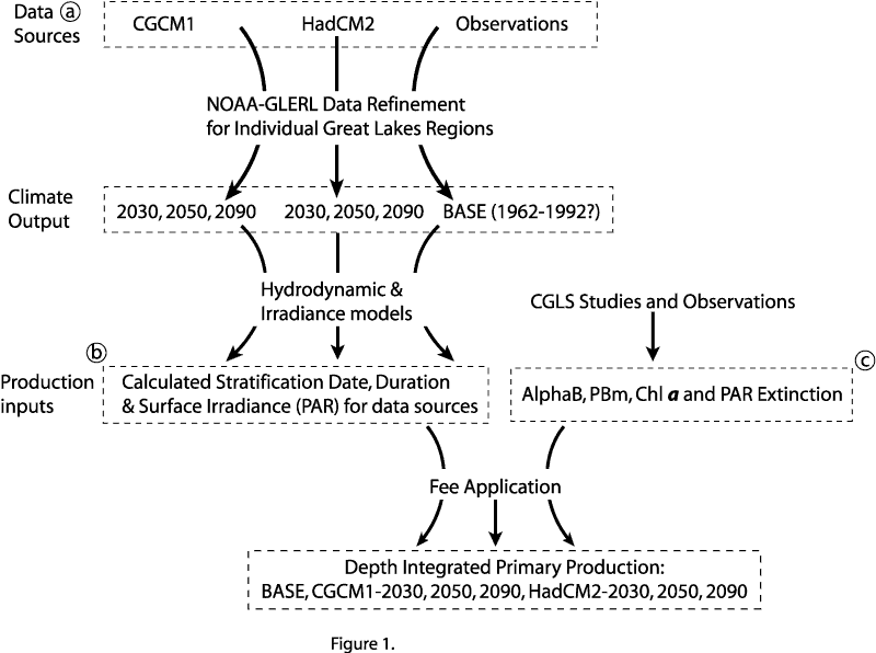
Figure 1. Data flowchart followed to determine projected phytoplankton production in Lake Michigan. a) This project was supplied with refined climate data for Lake Michigan, the processing of which is detailed in Loftgren et al. (2001this report). b) Thermal structure and surface irradiance was determined by the methods detailed in Lehman (2001this report). c)The biological inputs were averaged from multiple studies conducted at the University of Wisconsin Milwaukee, Center for Great Lakes Studies.
Physical information used for the BASE reference was derived from meteorological data for the Great Lakes region spanning the years 1961-1990 (Lofgren et al 2001 this issue). From these data monthly maximum, minimum and mean values for cloud cover and stratification dates were used to define the base conditions for Lake Michigan.
Output from two global climate models (GCMs) was prepared by the NOAA Great Lakes Environmental Research Laboratory (Lofgren et al 2001, this issue). Each model produced a set of physical forcing functions for three time periods centered about the years 2030, 2050 and 2090. The two models, described by Sousounis, (2001 this issue), were the Canadian Global Coupled Mode 1 (CGCM1) and the Hadley Centre Coupled Model v2, (HadCM2). The latter utilized more input variables specific to the Great Lakes region than the CGCM1. The resolution of both GCMs was such that only two grid cells covered the whole of Lake Michigan. Data generated for these cells that projected future climate conditions were averaged to generate a composite result for the entire basin.
We recognize that differences exist between nearshore and offshore areas of the lake and over longitudinal gradients, however, these model projections were the best available at the time of this study. The physical modeling provided a single date of stratification for the entire lake, which was a necessary simplification of the known, complex seasonal thermal structure. For example, northern sections of Lake Michigan are known to stratify later in the season than more southerly locations (Bolgrien and Brooks 1993) and nearshore areas warm and cool more rapidly than offshore regions (Brooks et al 1990, Brooks and Sandgren 1995).
Data from the climate models were used by Lehman (2001 this issue) to derive input variables needed for primary production calculations. The physical variables derived from the GCMs used for the calculations were the initial date and duration of whole-lake stratification, mixing depth and monthly average photosynthetically available radiation (PAR) at ground level.
Daily solar irradiance data were generated by scaling half-hour cloudless irradiance curves from Fee (1990) for latitude N 43 , to match the monthly average value predicted by the GCM-forced calculations. The derivation of total incident short wave radiation data is presented by Lehman (2001, this issue). These monthly values were then linearly interpolated at two-week intervals. A comparison of irradiance values calculated using BASE data and data recorded hourly at the Center for Great Lakes Studies in Milwaukee from April 1996 to June 2000 show good agreement (Figure 2).
[Figure 2] [Caption] Figure 2. Monthly average irradiance at ground level calculated for BASE mean and
BASE minimum and maximum cloud cover conditions over Lake Michigan. Daily average observed irradiance was obtained
from hourly data (April 1996 through June 2000) at the Center for Great Lakes Studies, Milwaukee, WI.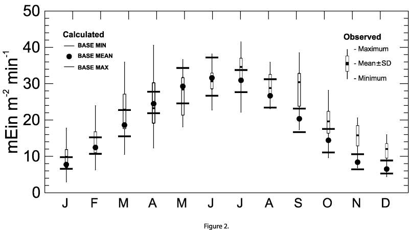
The sub-surface light extinction data and the biological variables required as input for the calculation of integrated primary production using the Fee application (Fee, 1990,1998) were derived from numerous studies at a 100m deep station in Lake Michigan, referenced as Fox Point (W87.65, N43.22) (Table 1). These studies spanned a period from 1985 through 1999 (Brooks et al 1990, Brooks and Sandgren1995 and Center for Great Lakes Studies monitoring cruises R. Cuhel, personal communication). Sub-surface light intensity data observed at Fox Point were entered for depths of 5, 10, 20 and 30 m and interpolated programmatically over time and depth for the indicated segments of the water column using the methods described by Fee (1990, 1998).
Although there are few values for the biological input variables reported in the literature for fall through early spring, published values for summer conditions (Fahnenstiel and Scavia 1987) are comparable with those used here for the stratified season.
Aerial primary production for a one square meter column of water was calculated using the computer applications developed by Fee (1990) and updated on the WEB (Fee 1998). Daily integral photosynthesis was determined with program default settings (e.g. resolution of interpolation) using values describing the vertical light gradient, chlorophyll a and photosynthesis versus irradiance relationships.
The calculations of primary production for projected climate change scenarios were made using two different procedures. Initial calculations were run using the GCM-based projected physical conditions for the lake, but with mean BASE alpha and Pmax input values of 6.5 mg C mg chl a 1 Ein m 2 and 2.8 mg C hr-1 respectively, that did not change seasonally. Chlorophyll a input values ranged from 0.5 to 3 mg m-3 and followed seasonal BASE data. The second method utilized seasonal BASE P vs I inputs adjusted for projected changes in physical conditions in the lake. For example, under BASE conditions just prior to summer stratification a relatively high concentration of chlorophyll is vertically homogeneous throughout the water column, while after stratification surface chlorophyll values decrease and a sub-thermocline chlorophyll peak begins to develop (Brooks and Torke 1977). If the date of stratification was projected to occur earlier than the mean BASE date, post-stratification BASE biological conditions were imposed on the production calculation as of the projected date of stratification.
Results
Base-Year Production
Primary production calculations determined using the mean observational BASE data and biological data from the Fox Point station showed that the spring bloom commenced in March when the lake was fully mixed, increased rapidly through April and declined following stratification on or about June 13 (Figure 3). The rising limb of the curve during spring mixing reflected the increase in PAR as the season progressed. During this period, PAR levels were under saturating for optimal photosynthesis (<Ik) at depths >10m, while most of the algal biomass (measured as chlorophyll a) was below that depth. Following thermal stratification and the cessation of full vertical mixing, production declined. A slight pulse in production occurred just after stratification that may be attributed to increased chlorophyll in the sub-thermocline strata and continuing increases in PAR input through the summer solstice. Another pulse was observed in late October coincident with fall overturn. This pulse was short lived, however, due to diminishing PAR values as winter approached. Low light inhibited production throughout the winter months even though the water column was fully mixed and nutrients were abundant.
Under these conditions, mean base annual primary production was estimated to be 116 g C m-2. The range of production values as influenced by BASE minimum and maximum cloud cover, which results in maximal and minimal PAR, were shown to be 129 and 104 g C m-2 respectively (Table 2).
[Figure
3] Figure 3. Calculated primary production using BASE light scenarios and mean historical photosynthetic
parameters. The area between the vertical dashed lines represents the period of thermal stratification under
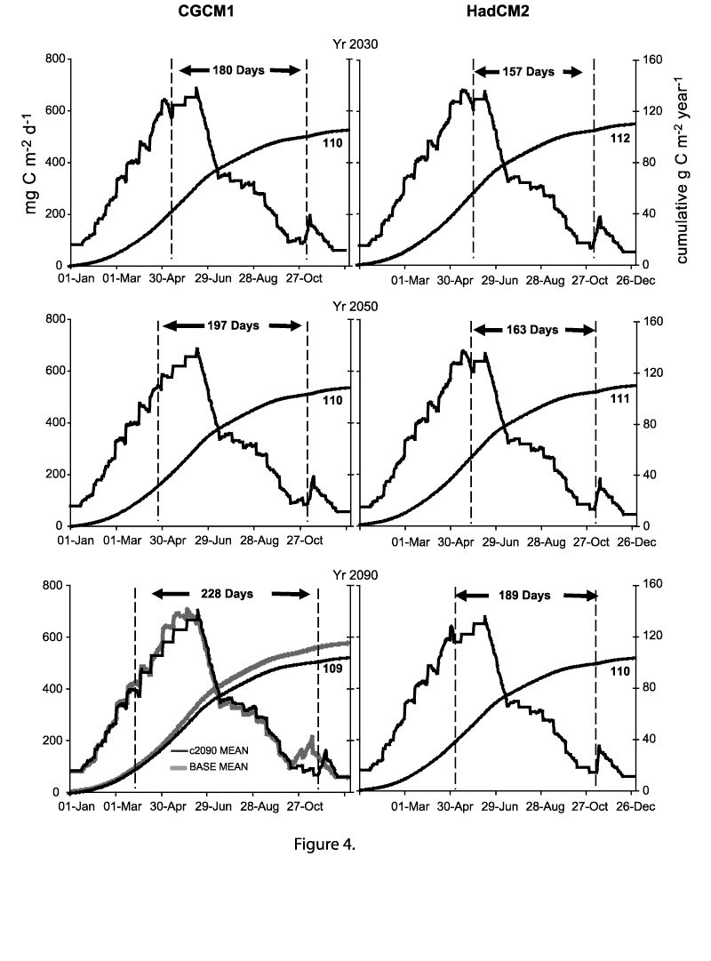
BASE conditions. Figure 4. Daily (stepped plot) and cumulative annual (smooth curve) primary production for
Lake Michigan calculated using projected physical conditions derived from the Canadian
Climate Centre (CGCM1) and Hadley (HadCM2) global climate models, and BASE biological variables
adjusted for the estimated climate change for the years 2030, 2050 and 2090.
The area between the vertical dashed lines represents the projected period of thermal stratification.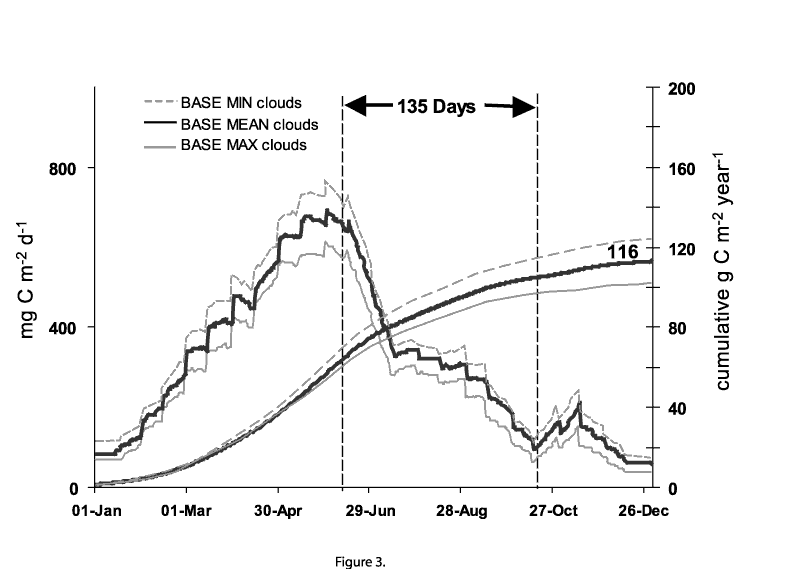
Projected Production
Primary production calculated using mean annual P vs. I input factors that were not changed seasonally, and the mean stratification and cloud cover conditions projected for the year 2090 are superimposed on the base production data illustrated in Figure 3. These data show the effect of the earliest projected date of spring stratification and the latest date of fall overturn (Table 2). Under these conditions annual primary production was projected to decline to 100 g C m-2 yr-1, a decrease of 14% from BASE values. These production calculations illustrate the hypothesized influence of changes in the duration of thermal stratification in Lake Michigan, independent of biological variability. The greatest loss of production occurred during spring with the early truncation of the spring bloom, while the later overturn in fall delayed the upward mixing of nutrients to a date when insufficient light was present to support the fall pulse shown under BASE conditions.
Primary production calculated using mean annual biological input factors that were changed seasonally according to the mean stratification and cloud cover conditions projected for the years 2030, 2050 and 2090 are illustrated in Figure 4. Both daily production estimates and cumulative values over the year are plotted. In comparison to the BASE conditions with a mean annual production of 116 g C m-2, projected annual production calculated with mean outputs from the HADCM2 model show a decrease in primary production of about 2% in 2030, 2% in 2050 and 3% by 2090 (Table 2). The CCM1 model projections resulted in decreases of approximately 3% in 2030, 2050 and 2090. Using the maximum cloud cover projected for 2090, annual production could decrease by approximately 13% to 101 g C m-2 yr-1, whereas, with minimum clouds, production was projected to increase 7% above the BASE value.
DISCUSSION
The anticipated changes in the physical characteristics of Lake Michigan may impact primary production in two ways, both of which are related to incoming solar radiation. First, altered light intensity, due to an increase or decrease in cloud cover, would directly influence rates of photosynthesis. Second, changes in incoming solar radiation could alter surface warming and the thermal structure of the lake by extending or retarding the onset and ending dates of stratification (McCormick 1990). Other meteorological variables, such as wind and precipitation would also be important in determining the physical characteristics of the lake (Lehman 2001 this issue) and/or the overall hydrology and runoff inputs to the lake (Lofgren et al 2001 this issue). Both GCMs used here suggest a warming of the lake and longer periods of stratification, starting earlier in the spring and extending later into the fall.
The biological implications of the physical changes predicted by the climate models suggest that for Lake Michigan the extended duration of thermal stratification will reduce the duration of winter-spring mixing. Given that most algal biomass is produced during the spring bloom under well lit, vertically mixed, nutrient-replete conditions, any diminution of the mixed period would be expected to reduce the amount of primary biomass produced. Scavia et al. (1986) noted inter-annual decreases in algal biomass caused by a shortened mixing period resulting from extensive ice cover. Brooks and Torke (1977) reported that chlorophyll a was reduced by as much as 40% at the end of the spring bloom in 1974 when stratification occurred 6 weeks earlier than that observed in the previous year. Such changes may be indicative of future conditions under projected climatic change scenarios.
The BASE scenario that was determined from recent observations of the lake represent the coolest conditions and the shortest period of thermal stratification considered in this study. Under this scenario, the mean date for the onset of thermal stratification was June 13, just prior to the summer solstice, and extended for135 days through October 26. The mean BASE annual production of 116 g C m-2, calculated for these conditions, is comparable to published values for Lake Michigan (Fahnenstiel et al 1989, Fahnenstiel and Scavia 1986).
The projected extension of stratification into the spring bloom period was hypothesized to limit the bloom by placing a cap on the reservoir of nutrients in the sediments that are carried into the euphotic zone during spring mixing (Brooks and Edgington 1994).
A similar phenomenon was assumed to occur in fall when stratification was projected to extend beyond the date at which light could support production in the fully mixed water column. In other words in the fall, if mixing and the release of nutrients from the bottom waters did not commence until after the critical depth for light (Sverdrup 1953) rose above the depth of mixing, there would be no net production realized at the time of fall overturn. These reductions of the spring and to a lesser extent the fall algal blooms, coupled with projected changes in cloud cover, appear to be the principal causes of the climate-induced changes in primary production.
The significance of light variance alone, to an otherwise identical annual production calculation, indicated that BASE production varied 10% when the surface irradiance was modified using maximum and minimum cloud conditions. Similar ranges were also seen about the means of projected production under altered climate scenarios (Table 2).
The influence of the most extreme climate projections on primary production are shown in data plotted for the year 2090 using projections from CGCM1 (Figure 3, 4 and Table 2). Under this scenario stratification was projected to occur on April 5 and extend for 225 days through November 20. The extended period of stratification, as compared with BASE conditions, reduced the spring and fall production pulses when both the annual mean biological input variables were used (Figure 3) and when they were varied seasonally (Figure 4). In spring, early stratification was assumed to have imposed limiting conditions on the phytoplankton. This was not as apparent as initially expected, however, as production continued to climb after the projected date of stratification.
The continued increase in PAR beyond the early projected date of thermal stratification appears to have strongly influenced the primary production calculations independent of any limitation imposed by the application of post-stratification P vs. I input variables indicative of nutrient limitation, such as a lower Pbm. This is not unexpected given that mean light levels at depths >10 m were estimated to still be less than saturating values at the projected date of early stratification in early April. Any increase in PAR beyond that date would be expected to result in increased production. As PAR data input to the production calculation continued to increase, the production estimates followed until light began to diminish in late June. For example, daily average scalar irradiance at 10 m for January 1 under BASE conditions was 32 mmol photons m-2 sec-1 and saturating light intensity at the same depth (Ik) was 69. By June 24, that value increased to an annual maximum of 110, and the June Ik was 117 mmol photons m-2 sec-1. These numbers simply illustrate that for most of the year, irradiance at about 10 m and below is sub-saturating and phytoplankton production would be sensitive to increases or decreases in light at or below about 10 m. For reference, the BASE annual average Ik at 10 m in this study was 116 (annual SD = 49). Annual Ik calculated from Fahnenstiel for Lake Michigan (1989) were 108 (annual SD = 21).
Although the availability of nutrients does not directly influence the production calculations presented here, with such an early date of stratification projected the reservoir of nutrients remaining in the surface waters after stratification would be expected to be greater than if the bloom had been allowed to continue later into the spring. Normally, under BASE conditions with stratification occurring in mid-June after an extended period of mixing and production, nitrogen and silicon would be diminished leaving little reserve for further production in the surface waters (Brooks and Edgington 1994). With the earlier projected date of stratification, this reserve would be greater and could continue to fuel the spring bloom for a time after stratification had occurred as PAR continued to increase. In fall the extended period of stratification would delay the upward mixing of nutrients that occurs at overturn to a date beyond which light could support any new production in the fully mixed water column.
The results of this research suggest that primary production in Lake Michigan will decline as climate warms. This decline will occur principally as a result of increased duration of thermal stratification that will limit the availability of nutrients in the lighted euphotic zone of the lake. When these primary production results are coupled with the estimates of zooplankton abundance and fishery yield developed by Hill and Magnuson (1990), they suggest if the productivity of the lower food web is diminished, then fishery production will also decline. The magnitude of the fishery decline will require more detailed study of the intermediate links in the food web to better understand the complexities of the system.
Compounding these predictions are unknowns, such as changes in primary producer metabolism resulting from warmer conditions, possible algal species shifts, changes in tributary runoff and nutrient inputs and the invasion or introduction of new exotic species that could completely change the structure of the food web as we know it today. Changes brought about by exotic species have been well documented in the past with the invasion of the alewife, sea lamprey, gobies, zebra mussels, Bythotrephes and the stocking of exotic salmon. The effects of climate change alone on the biological productivity of the Great Lakes would appear to be the easiest to predict in the face of unknown invaders and to changes related to politically-driven fishery management decisions.
The scientific community must respond to climate change with an observational program that can detect the strengths and weaknesses of these and other predictions. Studies will be required that integrate the results of research conducted in many disciplines. Critical to our understanding of the food web in the lakes will be knowledge of changing cloud cover and wind patterns that may alter irradiance, nutrient dynamics, thermal cycles and mixing patterns in the lakes. Links in the food web between the primary producers and the top, economically important fish in the system must also be examined in greater detail.
While there is much to be gained by effectively monitoring present conditions, much knowledge can be gained by looking back at extant historical records. The collection of good quality data at frequent intervals will aid in addressing the research needs outlined above, while the analysis of past conditions may elucidate inter-annual variance and extreme events that will strengthen the validity of longer-term climate-coupled projections.
ACKNOWLEDGMENTS
REFERENCES
Blumburg, A.F. and D.M. Di Toro. 1990. Effects of climate warming on dissolved oxygen concentrations in Lake Erie. Trans. Am. Fish. Soc. 119:210-213
Bolgrien, D.W. and A.S. Brooks. 1992. Analysis of thermal features of Lake Michigan from AVHRR satellite images. J. Great Lakes Res. 18:259-266.
Brooks, A.S. and C.D. Sandgren 1995. Nearshore Hydrodynamics Affecting the Lake Michigan Coastal Waters of Wisconsin: Biological Productivity Along Thermal Fronts in Coastal Waters. Final report to. NOAA Great Lakes Environmental Research Laboratory, Ann Arbor, MI.
Brooks, A.S. and D.N. Edgington. 1994. Biogeochemical control of phosphorus cycling and primary production in Lake Michigan. Limnol. Oceanogr 39: 961-968
Brooks, A.S. et al. 1990. Algal productivity measurements at Great Lakes water intakes. Final report to Great Lakes National Program Office, U.S. Environmental Protection Agency, Chicago, IL
Brooks, A.S. and B. G. Torke. 1977. Vertical and seasonal distribution of chlorophyll a in Lake Michigan. J. Fish Res. Bd. Can. 34(12): 2281-2287
Fahnenstiel, G. L. J. F. Chandler, H. J. Carrick and D. Scavia, 1989: Photosynthetic characteristics of phytoplankton communities in Lakes Huron and Michigan: P-I parameters and end-products. J. Great Lakes Res., 15: 394-407.
Fahnenstiel, G.L. and D. Scavia, 1986: Dynamics of Lake Michigan phytoplankton: primary production and growth. Can. J. Fish. Aquat. Sci. 44: 499-508.
Fee, E.J. 1990. Computer Programs for Calculating In Situ Phytoplankton Photosynthesis. Can. Tech. Rept. Fisheries and Aquatic Sci. 1740
-------- 1998 Revision of 1990 Computer Program for Calculating in-situ Phytoplankton Photosynthesis. At: http://www.umanitoba.ca/institutes/fisheries/PSpgms.html
Hill, D. and J.J. Magnuson, 1990: Potential effects of global climate warming on the growth and prey consumption of Great Lakes fish. Trans. Am. Fish. Soc.119: 265-275.
Lehman, J.T. 2001. Mixing dynamics and plankton biomass of the St. Lawrence Great Lakes under climate change scenarios. J. Great Lakes Res. (This issue)
Lofgren, B.M. F.H. Quinn, A. H. Clites and R. A. Assel. 2001. Climate change impacts on Great Lakes basin water resources. J. Great Lakes Res. (This issue)
McCormick, M.J., 1990: Potential changes in thermal structure and cycle of Lake Michigan due to global warming. Trans. Am. Fish. Soc.119:183-194.
Magnuson, J.J., J.D. Meisner and D.K. Hill, 1990: Potential changes in the thermal habitat of Great Lakes fish after global climate warming. Trans. Am. Fish. Soc. 119: 254-264.
Meisner, D.J., J. L. Goodier, H. A. Regier, B.J. Shutter and J. Christie. 1987. An assessment of the effects of climate warming on Great Lakes basin fishes. J. Great Lakes Res. 13:340-352.
Rowe, G.T. and J. G. Baldauf, 1995: Biofeedback in the ocean in response to climate change. 233-245. Biotic feedbacks in the global climatic system. G.M. Woodwell and F. T. Makcenzie eds. Oxford Univ. Press 416 p.
Scavia, D, G.L. Fahnenstiel, M.S. Evans, D.J. Jude and J.T. Lehman, 1986: Influence of salmonine predation and weather on long-term water quality trends in Lake Michigan. Can. J. Fish. Aquat. Sci. 43: 435-443.
Smith, S.V., 1995. Net carbon metabolism of oceanic margins and estuaries. 246-250. Biotic feedbacks in the global climatic system. G.M. Woodwell and F.T. Makcenzie eds. Oxford Univ. Press 416 p.
Sverdrup, H. U. 1953. On conditions for the vernal blooming of phytoplankton.
J. Cons. Explor. Mer, 18, 287-295.
Woods, J. and W. Barkmann, 1993: The plankton multiplier positive feedback in the greenhouse. J. Plankton Res. 15: 1053-1074.