|
Site Home
PHOTOACCLIMATION
OF THE DIATOM ASTERIONELLA FORMOSA
IN A SIMULATED
VERTICALLY MIXED WATER COLUMN
By
John C.
Zastrow
The University
of Wisconsin � Milwaukee, 2001
Under the
Supervision of Professor Arthur S. Brooks
ABSTRACT
A
clone of the diatom Asterionella formosa was studied to determine
the ability of the species to photoacclimate as they were passed
through a light gradient at varying rates. Columnar incubators 4
m in height, held at 4 � C, with a light gradient of 250 �
10 mmol photons m-2 sec-1
were used to simulate vertical mixing as found in Lake Michigan.
Asterionella
formosa used both increases in the number and size of photosynthetic
units to acclimate to lower irradiances. These increases occurred
within 24 hours of being introduced into a new light climate, though
clear trends in the response of photosynthetic parameters and pigments
to light history was tenuous in two of three experiments. In general,
the photoacclimation response included synthesis of photosynthetic
pigments that appeared to be proportional to each other across all
light histories and maximal intensities. This proportionality in
pigmentation included samples taken from the darker and bluer BOT
treatments, where the potential for chromatic adaptation to alter
pigment ratios was highest. However, after one week the cells in
the BOT treatment became so light limited that they were incapable
of synthesizing pigment and the cell density began to decline. This
indicates that cells require certain total daily or weekly light
dose in order to successfully photoacclimate to reduced light conditions.
Contrary
to published trends, the TOP samples in all experiments increased
or maintained chlorophyll content despite being in light at non-limiting
intensities. It appeared that the cells needed to add chlorophyll
until they approached a maximum of about 2.5 pg cell-1,
where cells in experiment 0205 seemed to maintain their content.
The final experiment yielded the most consistent evidence of periodic
photoacclimation that was correlated with daily light history. The
fact that this periodic acclimation only became apparent after ten
days under the mixed light regime suggests that acclimation to a
non-diel, cyclic light cycle may be occurring.
Abstract iii
Acknowledgements. v
Table of contents. v
List of figures. vii
List of tables. viii
Introduction. 1
Photoacclimation. 1
Objectives. 6
Methods. 7
Isolation
and culturing. 7
Experimental
columns. 9
Experimental
Incubations. 16
Cell
counting and particle corrections. 17
Pigment
extraction and analysis.
19
Photosynthetic
parameters. 25
Results. 28
Growth
rates. 29
Pigmentation. 34
Photosynthetic
capacity and efficiency. 35
Discussion. 45
Photoacclimation
in pigmentation. 45
Photoacclimation
in photosynthesis.
47
Influences
of temperature and diel periodcity on photosynthesis.
50
Implications
for in situ primary production. 51
Conclusion. 54
Bibliography. 56
Appendix. 61
Appendix
A. Cell counts and growth rates. 61
Appendix
B. Pigments. 62
Appendix
B, cont.63
Appendix
C. Pigment correlations.
64
Appendix
D. Pigment TDLD regression results. 65
Appendix
E. Photosynthetic parameters modeled with Platt, 1976.
66
Appendix
F. Photosynthetic parameters modeled with Fee application.
67
Appendix
G.DYV Freshwater Phytoplankton Medium.. 68
Appendix
H. Photosynthetron SOP.
69
Appendix
I. Background for DATPARSE Beckman scintillation parsing program.. 70
Appendix
J. Background on the stepping motor71
Figure
1. Asterionella formosa. Image taken from a field sample at 40x.7
Figure
2. Experimental columns.10
Figure
3. Light sensors.12
Figure
4. Comparison of sensor response to irradiance.13
Figure
5. Measured and calculated PAR versus light intensity.14
Figure
6. Bottle clamp used to fasten sample bottles to the suspension
lines in the columns.16
Figure
7. Example of particle size and colony size distributions.18
Figure
8a. Example spectrophotometric scans of pigments in 90:10 acetone
: water.21
Figure
8b. Spectra in SCOR eluant after HPLC separation.22
Figure
9. Photosynthetically available radiation received by each treatment.30
Figure
10. Cell densities determined by particle counter30
Figure
11. Cell density versus cumulative light exposure.32
Figure
12. In vitro whole sample and cell-specific chlorophyll a.33
Figure
13 a, b and c. Photosynthesis versus irradiance plots.35
Figure
14a, b, and c. cell-specific photosynthetic parameters.42
Figure
15 a, b, c. Chlorophyll-cell specific photosynthetic parameters.43
Figure
15 d, e, f. Cell-specific photosynthetic parameters.44
Figure
16. Pmax versus the daily summation of photons for each
bottle incubated under mixing conditions.48
Figure
17. Cell-specific photosynthetic parameters aggregated by treatment
versus the daily summation of photons.49
Figure
18. Light profile for Fox Point station during the spring of 1987.53
Figure
19. Treatment means from experiments 0226 and 0325 experiments versus
total daily light dose.54
Table
1: Culture medium composition.
8
Table
2. One-way ANOVA with Tukey post hoc of 0325 MIX samples by TDLD.. 40
Table
3. Summary statistics for the comparison of photosynthetic parameters
and pigmentation effects.41
Table
of Contents
Introduction
Pelagic
phytoplankton communities in the oceans and in large, deep lakes,
such the Laurentian Great Lakes, are strongly influenced by vertical
mixing processes. This turbulent physical process controls the availability
of nutrients (Brooks and Edgington 1994), the light to which the
cells are exposed (Falkowski and Raven 1997), and distribution
of the organisms themselves (Reynolds 1998). The interaction of
location-imposed resource constraints forces phytoplankton to constantly
optimize life processes. Photosynthesis is a critical life
process for photoautotrophic organisms and is modulated, within
a single cell, in a changing light environment via photoacclimation.
One
major effect that vertical water movement has on phytoplankton is
to force the cells through a light gradient. As attenuation of light
increases, the gradient becomes steeper through shading from living
and non-living particles and substances (Grobbelaar et al.
1992).
The
rate of vertical transport and the direction of cell movement through
the water column of lakes and oceans dictates the rate and specific
physiological response of phytoplankton to a changing light environment.
If the mixing time is greater than the time it takes a community
to acclimate to the light at that depth, a vertical gradient of
some photoacclimation parameter will form. On the other hand, if
the time of mixing is less, the parameter will be uniform across
the region of transport. No clearly stated values for mixing velocities
in the euphotic zone of Lake Michigan could be found. However, for
perspective, results from the Marine Boundary Layer Experiment off
the coast of Monterey, California describe measured mixing velocities
associated with Langmuir circulations (Farmer et al. 1998).
They found maximal mixing rates of 10 cm sec-1 and averages
of 4-8 cm sec-1 at 15 m depth in response to average
wind velocities of 15.9 m sec-1 (30.9 knots) for two
days. At the mean mixing rates, the time for a parcel of water to
traverse the 15 m would be approximately 3 to 6 minutes.
As
the depth of mixing increases, the average light intensity that
the cells are exposed to will decrease. Therefore, as a community,
the rate of photosynthesis integrated over the depth of the water
column will decrease. However, the rate of respiration of the phytoplankton
population is largely independent of mixing depth (Li and Garrett
1998). Therefore, there exists a critical depth below which the
consumption of carbon by respiration is greater than that gained
by photosynthesis and a net loss of community biomass occurs (see
(Platt et al. 1991; Sverdrup 1953). The ability of a phytoplankton
community to photoacclimate extends the critical depth and ultimately
enhances net biomass production. A phytoplankton community that
is light limited should benefit greatly from a small degree of photoacclimation,
in terms of annual primary production.
The
processes of photoacclimation have been studied both experimentally
in marine environments, (Falkowski 1983; Gallegos and Platt
1982; Lewis et al. 1984a; Lewis et al. 1984b; Yoder
and Bishop 1985) and theoretically (Cullen and Lewis 1988; Dusenberry
2000; Eilers and Peeters 1988; Falkowski and Wirick 1981). The ability
to photoacclimate is ubiquitous throughout photoautotrophic plankton.
However, the mechanisms and rates can vary between taxa. The following
description presents some of the photoacclimation responses that
are common in many taxa (Falkowski and La Roche 1991). In
response to changes in photon flux density (light intensity) and
spectral quality, morphological photoacclimation can be manifested
by changes in cell volume, the number and density of thylakoids
membranes (Berner et al. 1989; Post et al. 1984) the
size of storage bodies (Sukenik et al. 1987) and changes
in the number or size of plastids per cell. Physiological changes
can include changes in lipid and pigment content as well as composition
(Falkowski and Owens 1980; Perry et al. 1981; Prezelin and
Alberte 1978). These physiological changes occur to minimize quantum
requirements for photosynthetic oxygen evolution (Dubinsky et
al. 1986), respiration (Falkowski et al. 1985; Geider
et al. 1986; Langdon 1987) and growth rate (Falkowski et
al. 1985; Laws and Bannister 1980; Post et al. 1984).
Though they can be subtle and difficult to quantify, cellular modifications
occur over a cell�s generation (Cullen and Lewis 1988) and should
not be confused with adaptation, which occurs over multiple generations
(Falkowski and La Roche 1991).
Phytoplankton physiological
responses to changes in light intensity can also be accompanied
by concurrent changes in metabolic priorities. The effect is well
documented and numerous studies of cellular kinetics describe shifts
in metabolic resource allocation based upon recent light histories
of phytoplankton (Cuhel et al. 1984). For example, Dunaliella
tertiolecta exhibits a rapid (<24 hour) diversion of lipid
and carbohydrate biosynthesis to double their light harvesting chlorophyll
protein complexes (LHCP) in response to a reduction in ambient light
(Sukenik et al. 1990). Shortly after LHCP allocation begins,
photosynthetic reaction center proteins (D1 and D2) accumulate.
Once these light reaction proteins have increased, carbon metabolism
shifts back to lipid production to allow for the construction of
additional thylakoid membranes. These new membranes provide room
for additional photosynthetic protein complexes. Each progression
has been modeled with first order kinetics (Falkowski 1984;
Hoffman and Senger 1988; Sukenik et al., 1990), though alternative
models have been proposed (Cullen and Lewis, 1988). This adjustment
to lower irradiances is not precise. For example, some compounds
may be generated in excess amounts before achieving a steady state
in relation to the light environment (Falkowski 1984a; Falkowski
1984b).
When
cells return to higher irradiances, resources are diverted from
protein production and allocated to lipids and carbohydrates (Sukenik
et al. 1990). The additional carbohydrates and lipids allow
the cell to rapidly increase in volume without the need for high
concentrations of pigment. Cell growth, both in numbers and in volume,
will dilute cellular pigment content. Of course, controlled reductions
of photopigment does occur and is not always simply a result of
dilution. Experiments using D. tertiolecta indicated that
about half of the reduction in pigment was due to dilution by increased
cell volume. The remaining reduction was likely due to direct decomposition
(Falkowski 1984a). Of interest to this study, is the change
in the relative amounts of specific photosynthetic pigments as the
cells modify their photosynthetic apparatus.
Acclimation
to changes in light intensity is overlaid with the intrinsic circadian
cycles found in all natural populations of phytoplankton (Prezelin
and Sweeney 1977); (Falkowski and Owens 1980; Marra 1980). In studies
of acclimation it is important to differentiate between photoacclimation
and physiological acclimation to diel periodicity. Post et al.
(1984) found that the diatom Thalassiosira weisflogii achieved
maximal chlorophyll content in the middle of the photoperiod and
then declined before onset of the dark period. Also, cellular chlorophyll
levels were minimal around the mid-point of the dark period and
began to increase before light onset. These diel cycles were separate
from reproductive cycles and remained present throughout a full
range of light intensities.
In
her excellent review of diel periodicity, Prez�lin (1992) suggests
that the cellular developmental cycle in diatoms, �never appears
to couple to a biological clock�Some diatom cell division appears
to always occur throughout the light period.� However, studies of
multiple species of marine diatoms indicate that synchronized, diel
variation in the photosynthetic parameter Pmax may be
ubiquitous throughout the diatoms with peaks typically occurring
at the mid-point of the light period (Harding et al. 1981).
This appears to be confirmed by field studies of diatom-dominated
marine systems (Harding et al. 1982; Mac Caull and Platt
1977; Prezelin and Alberte 1978; Prezelin and Sweeney 1977). (Prezelin
1992)
Most
studies of photoacclimation and photoadaptation have been conducted
under conditions where cells are transferred abruptly between high
and low light intensities. For example, Anning et al. (Anning
et al. 2000) studied photoacclimation using parameters similar
to those in my study. They exposed the marine diatom Skeletonema
costatum to large, abrupt changes
in irradiance (50-1200 mmol photons m-2 sec-1) at 15 � C. Cells
adjusted to 50 mmols were found to have higher levels of fucoxanthin and chlorophyll
a, but lower diadinoxanthin and diatoxanthin. Cells
grown at 50 mmol photons were transferred to 1200 mmols
and within two days cellular fucoxanthin declined from ~ 3.0 pg
cell-1 to 0.5 and chlorophyll a from ~1.0 to 0.4
pg cell-1. Chlorophyll c1c2 followed similar trends as
fucoxanthin and chlorophyll a. After returning to 50 mmols, the
cultures returned to their previous pigment contents
within four days. b-carotene is a photoprotective pigment that is not coupled
to the photosynthetic reaction centers, and protects the cells from
photooxidative damage from the capture of excess photons in high-irradiance
(Neale and Richerson 1987). b-carotene was
also measured by Anning et al. (2000), but was
invariant throughout the study.
In
addition to b-cartotene, diatoms posses other
carotenoids that play photoprotective roles, such as the xanthophylls
diadinoxanthin and diatoxanthin (DD and DT). DD is thought to be
a precursor to fucoxanthin and is thought to allow more rapid photoacclimation
upon a cell�s return to low light (Goericke and Welschmeyer 1992;
Lohr and Wilhelm 1999). Cells that were accustomed to low light
would be sensitive to damage by excess excitation from high light
intensities, as their reaction centers would be numerous.
As expected, the photoprotective xanthophylls had inverse responses
to both fucoxanthin and chlorophylls. Anning felt the lack of response
by b-carotene was due to the rapid intervention of DD and DT.
Anning et al. (2000) also found that cell-specific Pmax
did not shift in response to changes in irradiance. However, chlorophyll-specific
light saturated rates of photosynthesis increased after exposure
to high light. The light-limited rates of photosynthesis, measured
by a
normalized
to chlorophyll a (aB) showed no temporal
variability throughout the study. Cell-specific
a
(acell) did change and
was greater in the shade-acclimated cells. These responses indicated
that changes in acell were due to modulations
of chlorophyll a content and that cell-specific chlorophyll
a concentrations are important for controlling light-limited
photosynthesis.
A
handful of marine studies have considered the complex nature of
photoacclimation when cells are passed through a light gradient.
(Marra 1978) in a field setting using mixing and light gradients
focused upon optimal photosynthetic rates in response to varied
light histories. The study described in this thesis is one
of a few to consider photoacclimation to a smoothly changing light
gradient in a laboratory setting (Flameling and Kromkamp 1997; Ibelings
et al. 1994; Kromkamp and Limbeek 1993; Kroon et al.
1992a; Kroon et al. 1992b).
A
study very similar to mine was published in 1997 using the chlorophyte
Scenedesmus protuberans (Flameling and Kromkamp 1997). They
exposed cells, at 20 � C, to oscillating light over
a range of 200
to ~10 mmol photons m-2
sec-1 at a periodicity of 1, 4 and 8 oscillations every
ten hours. In each of these trials, the total daily light dose (TDLD)
remained constant, but the time spent at peak intensity was modulated.
They found that, when corrected for cell size, chlorophyll content,
Chl a/b ratio, the chlorophyll-specific absorption cross-section
or the carotenoid-Chl a in vivo absorbance ratio did
not change throughout the study. They proposed that algae that do
not successfully photoacclimate to an oscillating light environment
would exhibit a reduced rate of daily-integrated photosynthesis
and would lose biomass.
For
S. protuberans, like Skeletonema costatum and Phaeocystis
globosa, they determined that it was not the total daily light
dose (TDLD) that determined PBmax, but rather
the daily maximal irradiance experienced by the algae. This is in
contrast to their findings that light-saturated photosynthesis normalized
to chlorophyll a (PBmax) in the diatoms
Thalassiosira weissflogii and Phaeodactylum tricornutum
and were not influenced by the daily maximal irradiance. Also,
they found that cells held in a fluctuating light environment did
not exhibit declines in aB compared with
those held in a
high light environment. This supports Anning et al. (2000)
finding that light-limited photosynthesis is controlled by changes
in chlorophyll a content per cell.
Though
there are many rates and strategies that a given algal group may
employ to photoacclimate, in general when light levels are reduced,
pigments and proteins for light harvesting chlorophyll protein complexes
(LHCPs) are produced. As light increases, maintenance of high
concentrations of photopigments is unnecessary and cells will reduce
their pigmentation.
As
a common member of freshwater pelagic communities, Asterionella
possesses critical preadaptations to allow it to be successful in
a deep-mixed water column (Reynolds 1998). Physiological features
such as the rate and degree of chlorophyll a production,
both absolutely and in relation to the accessory pigments allows
genera such as Planktothrix (cyanobacterium), Aulacoseira
(diatom) and Asterionella to be successful in pelagic systems.
For example, the chlorophyll:carotenoid ratio is a longstanding
index that can be used to determine the photosynthetic health of
phytoplankton (Margalef, 1958 as cited by Reynolds 1998). The adjustment
of pigment concentration/pigment ratios is a strategy that must
be employed by all phytoplankton when their light environment has
shifted for a sufficient time. However, it is important to note
that simply increasing chlorophyll does not linearly increase the
functional photosynthetic cross-section of the photon-collecting
antennas. (Margalef 1958)
A
linear increase in photosynthetic rate with added chlorophyll requires
that the additional chlorophyll be spread evenly throughout the
cell. Failure to distribute the chlorophyll results in increased
internal self-shading, an effect referred to as �package effect�.
Modulating package effect is a very important strategy for photoacclimation
and assays of this parameter can provide yet another descriptor
as to the state of light-regulated photosynthetic efficiency (Anning
et al. 2000; Falkowski and La Roche 1991; Falkowski and Raven
1997; Grobbelaar et al. 1996).
An
anatomical flexibility that helps define the degree of package effect
is intracellular migration of chloroplasts between a cell�s periphery
and its core. Plastid relocation in response to super-saturating
irradiances is a common and important photoprotective mechanism.
In planktonic cells with multiple and moveable chloroplasts, cell
size limits, but does not negate, the usefulness of this mechanism
(Long et al., 1994). Although no images were captured, I was able
to confirm that light-limited A. formosa cells positioned
their chloroplasts against the cell wall when grown in light below
~30 mmols. This distribution of chlorophyll was
not as apparent when viewing cells grown at ~100 mmols,
where the chloroplasts tended to be located along the midline of
the cell and appeared to overlap slightly.
When
diatoms are exposed to prolonged doses of high light, contraction
of the chromophores and chlorophyll cross-section areas occurs within
minutes to hours (Neale and Richerson 1987). Under quickly changing
conditions, the Asterionella genus has one or more chloroplasts
per cell that can be moved to different positions within the cell
cavity in response to light stress. However, the nature of
entrainment of phytoplankton in the flows of a vertically mixed
water column means that it is not likely that an entire population
of cells would be over exposed at any time (Reynolds, 1998). In
the studies mentioned above, and many others, members of the group
Bacillariophyceae (diatoms) are a common focus, although
no studies were found that examined Asterionella spp. in
the context of photoacclimation.
Consideration
of the specific strategy of A. formosa requires a knowledge
of its particular pigment compliment. In general, diatoms posses
chloroplasts that contain chlorophylls a, c1, c2
and fucoxanthin as the principle carotenoid. Also present is b
carotene which is important as a photoprotective pigment when irradiance
intensities exceed levels that the cell can safely capture and funnel
to the reactions centers (Flameling and Kromkamp 1997).
Currently, it is not clear if the rate of community photoacclimation
in Lake Michigan is rapid enough to allow detection; especially
within the surface mixed layer under stratified conditions. It is
possible that cells may simply maintain a modified photosynthetic
apparatus suited to a light environment averaged through the water
column they traverse.
Figures: literature examples
Photoacclimation
time course
Extended
PA time course
Photosynthetic
action spectra
Microscopic
analysis of photoacclimation changes
Figures: methods
Diagram
of control setup
Detail
of control setup
Diagram
of bottle attachment
Photo
of column tops
Photo
of column top and controls
Temperature
and light dataloggers on string with sample bottle
Column
bases
The
primary objective of this study was to characterize photoacclimation
in the diatom Asterionella formosa as it passes through a
light gradient similar to those found in nature. Due to the properties
of light propagation in an aquatic environment, changes in intensity
are always associated with changes in quality (Kirk 1996). Though
an important aspect of the physical environment, spectral changes
were not considered experimentally in this project.
As
part of the overall objective, I hoped to determine a rate of acclimation
in relation to the rate at which the cells were �mixed� or passed
through the light gradient. The methods for detecting this change
focused on cellular pigment concentrations and measurements of photosynthetic
efficiency and capacity. If photoacclimation was not detected for
each traversal of the light gradient, a secondary objective was
to determine if the cells were responding to their entrainment cycle
on a longer time scale.
It
was hypothesized that once transitioned from an intermediate light
intensity, cells will begin to immediately photoacclimate to their
new light environments. Cells exposed to higher light intensities
will reduce their photopigments and shift their carbon assimilation
to synthesize proteins for light harvesting complexes that allow
them to use the high rate of photon flux. Cells transitioned to
low light will increase their pigments and photoreceptor complexes
to become more efficient at capturing the now sparse photons. These
conditions were considered high-light and low-light controls for
responses seen under mixed conditions. Cells that are moved through
the light gradient should exhibit a moderated response that is bracketed
by the response seen by the high and low light controls.
Results
from previous studies using rapid and non-gradual shifts in irradiance
show that a should increase and Pmax
should
decrease in the cells as they are brought from high light to low
light. This physiological shift should also occur in cells in a
treatment that simulates movement across a light gradient, as in
vertical water column mixing. The reverse condition where a
decreases and Pmax increases should occur as cells move
from low light to high light.
Table
of Contents
Methods
Isolation
and culturing
During
March 2000 multiple monocultures of four species of diatoms were
grown from isolates taken from 5m depth at Fox Point station in
Lake Michigan (43� 11� 40� N, 87� 40� 11� W). Members of the genera
Synedra, Fragilaria, Cyclotella and Asterionella were grown
in small batch cultures. It was decided that the most versatile
species upon which to focus this study would be Asterionella
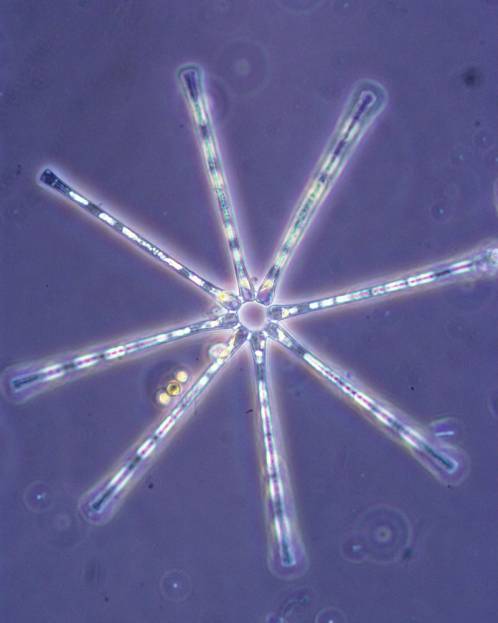
formosa (Figure 1). The star
shaped colonies were likely to yield accurate counts from the Coulter
particle counter and
Figure
1. Asterionella formosa. Image taken from a field sample at 40x.
(Image by Pat Eberland,
2000 REU program).
previous culture experience
suggested that A. formosa would be the easiest to maintain
in long-term batch cultures. The clone Aster8, which grew in culture
with the most vigor and reliability, was chosen for use in this
study.
Maintenance
cultures were grown in 150-mL, screw top Pyrex Erlenmeyer flasks
using the medium DYV ((Lehman 1976) as modified by Sandgren) (Table
1). The recipe was not altered and the final concentrations of nutrients
in media were intended to be non-limiting in all of the experiments.
Table 1: Culture medium
composition
|
Ingredient
|
Final
Medium Concentration
|
|
Calcium
chloride (CaCl2)
|
180
mM-Ca
|
|
Magnesium
sulfate (Mg(SO4)2 * 7H2O)
|
300
uM-Mg
|
|
Sodium
phosphate (Na2HPO4)
|
46.1
mM-PO4-P
|
|
Sodium
nitrate (NaNO3)
|
235
mM-NO3-N
|
|
Sodium
metasilicate (Na2SiO3 * 9H2O)
|
53.2
mM-Si
|
|
Ammonium
nitrate (NH4NO3)
|
125
mM-NO3
& 125 mM-NH4-N
|
|
Potassium
chloride (KCl)
|
134
mM-K
|
|
Sodium
bicarbonate (NaHCO3)
|
250
mM-C
|
Lighting
in the environmental chamber that held the maintenance cultures
was supplied by Cool White fluorescent bulbs at an average intensity
of 80 mmol photons m-2 sec-1
on a 12/12-light/dark cycle. Temperature was held at 10 �C.
Sub-samples
of the maintenance cultures were taken for use in the experiments.
Three to six weeks were required to grow as much as 30 liters of
log-phase culture and diluted to a density of about 2500 colonies
ml-1. Cultures were maintained in one-liter Nalgene polycarbonate
centrifuge bottles at 15 � C and 100 mmol
photons m-2 sec-1 supplied by Cool White High
Output (HO) fluorescent bulbs.
The
environmental chamber that provided sufficient space and lighting
to grow 30 liters of culture was unable to maintain temperatures
below 15 � C. Because the experiments were to be conducted
at 4 � C simulating a homothermal
Lake Michigan, I was concerned about damaging the cells with large
temperature changes. Therefore, the cultures grown at 15 � C were
diluted with media stored in the 10
� C chamber and mixed thoroughly in a 60-liter
carboy to reduce the potential for temperature shock at the start
of an experiment. The resulting mixture was then dispensed into
the polycarbonate sample bottles and left in the 10 �
C chamber overnight before being transferred to the 4 � C columns. In a later test, a sample bottle of media at 15 � C
cooled to 4 � C in approximately three hours when placed in a 4 � C water
bath.
Two
identical columnar incubators were used to create the light and
temperature conditions necessary for this experiment (Figure
2). Each column consisted of a gray PVC pipe measuring 33
cm in internal diameter and 4.0 meters tall. Each column was wrapped
with garden hose through which chilled water was circulated. The
pipe and wrapped hose assembly was jacketed with insulation. Vigorous
aeration was provided by an air stone at the bottom of each column
that kept the water homothermal from top to bottom and throughout
light and dark cycles. Testing using yo-yoing Onset Stowaway temperature
loggers showed that throughout the course of an experiment, and
at all depths, temperature did not deviate from the target 4.0 �
C by more than � 0.7 � C.
|
Figure
2.Experimental columns.
|
The left column
held static bottles at the bottom in ~ 5 mmol irradiance
(BOT) and at the surface in
~250 mmol (TOP). Bottles
in the right, MIX column were raised and lowered to simulate
cell movements through a natural light gradient.
|
Light was provided
by Sylvania Super Metal Arc 1000-watt lamps positioned directly
above each column, operating on 1 12/12 light/dark cycle. The desired
light intensity was
achieved by raising or lowering the lamp height above the columns.
The distance from the plane of the opening of the lamp shroud to
the surface of the water was 56 cm for all experiments and both
columns. The desired light intensity was achieved by raising or
lowering the lamp height.
The light conditions in the columns were measured using two data
logging instruments mounted on a single bracket, at the exact
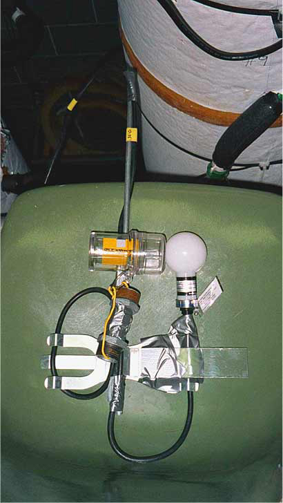
same level (Figure 3). One was
an Onset HLI light intensity logger, which is capable of recording
light intensity greater than normal room lighting. The other sensor
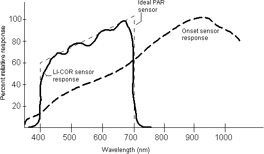
was a Licor scalar irradiance spherical sensor. The Licor sensor
records only radiation in the 400 � 700 nm region, while the Onset
HLI sensor records radiation somewhat below 400 and above 1000 nm(Figure
4).Each was set to begin logging at the same time and to
record light intensity at one-minute intervals. The sensors were
then lowered and raised in the columns at rates ranging from 10
to 1 cm min-1 to collect light readings continuously
over depth. The Licor sensor indicated that the light intensity
at 0.05 m below the water surface was 236 �
38 mmol photons m-2 sec-1with
the air stones on. Variance in this reading was likely due to the
influence of the pulsing light source, random scattering by the
bubbles and noise from the sensors. The light intensity at the bottom
of both columns with the air stones on was measured as 7 �
6
|
Figure
3. Light sensors.
|
|
An Onset HLI
light intensity logger (left) and a Licor spherical quantum
sensor (right) were used in logging mode to determine the
relationship of intensity versus PAR in the columns. The HLI
logger was attached to each mixed bottle cluster to log actual
PAR exposure throughout the experiment.
|
mmol
photons m-2 sec-1. Aeration diffused
and scattered the downwelling irradiance enough to increase attenuation
of light in comparison to un-aerated conditions.
The water in the columns
was chlorinated tap water that was changed at least every three
weeks to minimize the accumulation of particulates and biological
growth that would reduce the water clarity.
The
lamps did not produce constant light intensity over short time scales.
That is, a slight �pulsing� was observed both visually and with
light recording devices. These pulses would build and fade
with a period of less than 10 sec. and ranged as much as �
25 mmol photons m-2 sec-1 in surface irradiance.
To detect the pulsing with an instrument, the HLI logger was set
to record a measurement every five seconds without averaging. The
Licor logger was left to record average values sampled over 1 minute
and the intensity peaks were smoothed by this averaging.
In
each experiment where sample bottles were moved through a light
gradient an HLI light intensity logger was placed atop the cluster
of bottles to record the actual light history of the cells. Using
data from the Licor PAR scalar sensor, a conversion algorithm was
created to convert intensity values from the logger to apparent
scalar irradiance exposure using nonlinear fitting techniques such
as the following general model (Figure 5):
|
(Int)0.25 = HLIR
HLIR= a*PARm
b
|
(1)
|
where Int is
the light intensity measured by the HLI light logger in lumens and
PARm is the reading from the Licor spherical quantum sensor. The
fourth power transformation was used to reduce the heterogeneity
of variance in the readings from the HLI sensors. It is a known
property of the sensors that the amplitude of the noise increases
as the light intensity increases and this problem negatively influenced
the modeling. Conversion of the HLI readings, and the resulting
high-amplitude noise, to PAR often resulted in values that were
outside of the range observed by the Licor sensor. In the experimental
columns, with the bubbles and clean water, the following relationship
was found.
|
PAR = (HLIR/0.832163315)
(1/0.252975443)
|
(2)
|
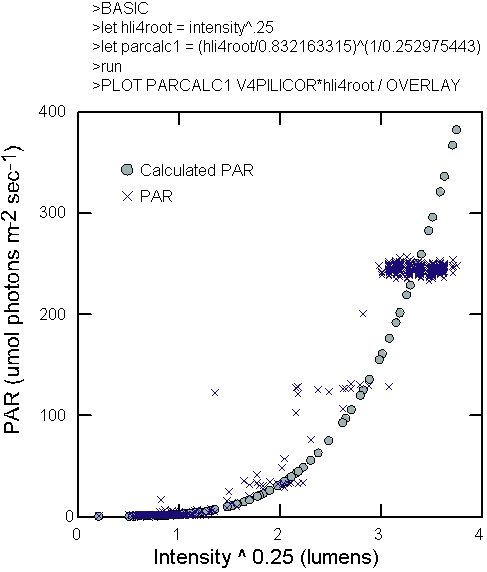
The light intensities
found in the columns approximate those found in Lake Michigan, during
mid to late spring, at depths of 1.5 to 16.5 meters.
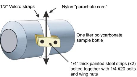
In
both columns, sample bottles were attached to nylon cord with adhesive-backed
1.25 cm Velcro straps and metal clamps. The adhesive side of white
Velcro was wrapped around each bottle leaving the facing side exposed.
Clamps consisting of two metal strips approximately 3.2 cm long
were held together using bolts and wing nuts. The clamps firmly
pinched the cord to the reciprocal half of the Velcro assembly so
that the bottle was securely attached to the line. The single point
of attachment allowed the bottles to rotate slightly about their
long axis when the cord was moved. Removing each bottle was simply
a case of disengaging the Velcro straps.
The
length of the metal strips, and hence the weight of the clamps,
was optimized to make each bottle only slightly negatively buoyant
when completely filled with medium. This was important to reduce
the amount of strain on the motors used in the incubators. White
Velcro, which was slightly translucent especially when wet, was used
instead of black to limit the
amount of shading in each bottle (Figure 6). For each
experiment, 12-15 bottles were placed at the position of each treatment.
Three replicate bottles were used for each sampling in all
experiments. For example, in experiments where there were MIX, TOP
and BOT treatments, 9 replicate bottles were sampled. The
physical diameter of each bottle meant that the replicate bottles
for each treatment spanned approximately one meter of column
depth in the TOP and BOT treatments, and about 0.5 meters for the
MIX treatments. I did not record the position of each bottle to
correct for light exposure during data processing.
As
stated earlier, the study used two nearly identical column incubators.
One was used as a �static� column where samples were left at the
top (TOP) and bottom (BOT) of the column throughout the experiment.
In the second column the sample bottles were moved up and down at
a fixed rate for each experiment (MIX).
The
mechanism employed to move the samples through the light gradient
used a stepping motor and drive (Intelligent Motion Systems Microlynx
7) with a program to control the travel rate, position at reversal
and to log the positions of the samples over time (Appendix J).The
stepping motor was mounted on a frame with
an arm that extended over the center of the MIX column. The stepping
motor was connected to an axel via a roller chain and sprocket gears.
Mounted on the axle were two fixed spools that rotated in tandem.
The suspending cord was wound around the spools such that a hanging
loop was formed in the column. The stepping motor, rotated in decimal
degree increments as specified by the program interface.
A
second motor and offset pulley rotated constantly to gently jostle
the bottle lines in both columns to keep the cells in suspension
in the sample bottles. This technique met with limited success and
the cells tended to settle after 24 hours despite the jostling.
At least every 24 hours, the bottles were agitated in the columns
to resuspend any settled cells. In addition, extreme care
was taken to gently mix the sample bottles prior to any sampling.
Experimental
Incubations
Four
experimental incubations were conducted for this study (experiment
numbers by date 1212, 0205, 0226, 0325). Three experiments were
conducted with mixing conditions (0205, 0226, 0325). One was without
a mixed sample and used only samples fixed at the top and bottom
of the column (1212). In experiments 0205 and 0325 the mixing samples
traversed the length of columns every 24 hours and had top and bottom
fixed controls. Experiment 0226 traversed the column length in 144
hours (6 days) and had a set of bottles in the environmental chamber
at 15 � C where the cultures
were kept. This treatment was simply to monitor for changes in the
replicates that were due to age alone. A seven-day acclimation period
was used in experiment 0325. This allowed cells to become adjusted
to their new light regime before sampling was started. In figure
9, the end of the acclimation period is day eight on the
horizontal axis. The other experiments did not undergo acclimation
in the columns prior to the sampling.
The
conditions for the study were originally chosen to maximize the
possibility of detecting photoacclimation. This study uses light
intensities that fall within those in the literature, including
static and mixed studies, where photoacclimation has been noted
in less than one photoperiod (12-8 hours). Also, this study allowed
the cells much longer time to acclimate to the changing light climate,
with gradient traversals of 24 hours or longer. Previous studies
cited in this thesis have moved cells through gradients with ranges
of scalar irradiance of 40-160, 15-167 and 30-320 mmol
photons m-2 sec-1. The same studies had traversal
times of 80 minutes (Kromkamp and Limbeek 1993) to two hours (Flameling
and Kromkamp 1997). The original study design called for additional
experiments to further refine the nature of acclimation by A.
formosa to the experimental conditions. However, mechanical
failures of the stepping motor prevented further experiments.
Previous
studies have cited detectable changes in many physiological parameters
due to diel cycles. Lacking the time to address these changes, I
opted to minimize their influence on the results and sample every
24 hours. Care was taken to not phototraumatize the cells by exposing
them to light that was outside their normal diel pattern. Therefore,
sampling was always conducted when the lights were off and cells
were �expecting� to be in the dark based upon a 12/12-light/dark
cycle. The cycle was synchronized between the column lights and
chamber lights. All experiments began or samples were taken before
07:00 or after 19:00. Once sampled, the only light that the cells
experienced was that of the photosynthetron. The time between
sampling and when samples were placed in the photosynthetron was
always less than two hours. The laboratory was dimly lit with red
lighting during all analyses for photosynthetic parameters and pigmentation.
Within
two hours of sampling, all replicate bottles were analyzed to determine
the number of cells per milliliter of sample, or the cell density
of the sample. All pigment and photosynthetic analyses were done
on a per cell basis, calculated using bulk parameters normalized
for cell density. Cell density was determined using a Coulter Multiziser
2 particle counter. Multiple samples from each replicate bottle
were counted and the average particle density was then corrected
for cell count. The correction was created by visually counting
the number of cells per colony in five samples. Visual observations
were made on live material at 40X magnification on a compound microscope
using a plain glass slide.
The
resulting histograms of the number of cells per colony were compared
to the distribution of particle sizes. A typical comparison is shown
in figure 7.
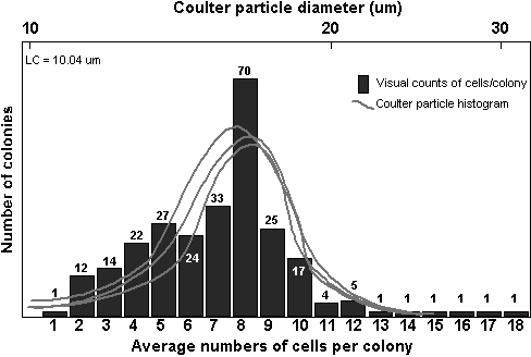
Through periodic visual
inspections, the only particles in the cultures in the size range
of 10 to 60 mm were cells and colonies of A.
formosa.
Therefore,
Coulter particle size frequency histograms in this range resulted
exclusively from differing colony sizes. While the cells of each
colony displayed some variance in size, it was reasoned that the
changes in colony size must be dominated by differences in the number
of cells per colony, and not differences in individual cell sizes
or morphologies. This would especially be true within each replicate
bottle. Under this assumption, the distribution of particle size
frequencies was then broken into groups, which represented a likely
number of cells per colony.
Three
to four particle counts for each replicate sample bottle were made.
Text files from the particle counter were imported into a spreadsheet
for conversion to cell densities per bottle. The particle/colony
size corrections were made for each count individually and the resulting
particle densities were averaged for each bottle.
Daily
specific growth rates for the duration of the sampling period were
calculated as follows:
|
Specific growth
rate = ln (N(T2)/N(T1))/(T2-T1)
|
(3)
|
where
N(T1) is the cell density at the start (T1) and N(T2)
is the density at the end of the study period (T2).
After
removal from the incubators, the samples were kept in darkness and
exposed only to dim, red lighting prior to filtration. Filtration
was performed using sintered glass filtration stands and Gelman
Supor 400 0.4 micrometers filters under 12 PSI of vacuum. Each stand
was rinsed once with deionized water between samples. Between experiments
the stands were soaked in 5% HCl then soaked in deionized water
and rinsed before drying. In this way, blockage of the sintered
glass surface was kept to a minimum.
After
some experimentation, the optimal volume filtered for pigment extraction
was determined. Of primary consideration was to keep the maximum
optical density near 1.0 in the scanning spectrophotometer. Allowing
the density to exceed 1.5 yielded too much noise in the response.
When the particle concentrations were on the order of 2500 � 3000
particles per milliliter (as determined in the Coulter counter within
the interval of 10-60 mm
diameter), 150 milliliters were filtered onto each 47mm filter.
If the particles densities fell below 2000, 200 milliliters were
filtered.
Two
filtrations for pigments were performed for each replicate bottle.
Each filter was immediately folded into quarters and stored in aluminum
foil packets in the freezer until the end of the experiment.
Following the experiment, the filters were extracted all at once.
Each filter was placed into 14.5 milliliters of 90% acetone buffered
with magnesium carbonate. The acetone was dispensed directly into
glass, 25-milliliter scintillation vials from a repeating dispenser
stored in the freezer. Each filter was then steeped in the freezer
for one week to maximize the extraction of accessory pigments. Rowan
(1989) determined that after seven days of steeping, no additional
significant pigment extraction would occur. Any disparity in terms
of the percent of pigment extracted from samples taken at either
end of experiments should not have produced any significant differences
in results. No grinding or sonication was used, as others have reported
sufficient extraction without these methods (Rowan 1989), Sandgren
(personal communication), Cuhel (personal communication).
After seven days the contents of each vial were poured into 15 mL,
graduated, screw top centrifuge tubes and centrifuged at 2500 RPMs
for 15 minutes to remove particulates. The supernatant was then
drawn off and stored in clean scintillation vials in the freezer.
Final volume of each extract was about 12 mL. The pigment
extracts were read in a Beckman 7000 DU diode array scanning spectrophotometer
with a 1nm bandwidth spectral resolution. The cuvette was a 10cm
quartz microcell with a glass lid to prevent evaporation during
analysis. The samples were scanned for absorbance at the 1nm resolution
from 360 to 760 nm, before and after acidification with 0.25 ml
0.1 N HCl (Figure 8a, b). Each sample generated two text files that
were imported into a spreadsheet for calculations.
Using
the methods presented by Arar (1997), which are based upon Jeffrey
and Humphrey's trichromatic equations, the concentrations of chlorophyll
a / pheophytin a and c1+c2 were calculated.
Chlorophyll b was not measured as it is not present in the
Bacillariophyceae(Rowan 1989). The basic equations
used in these calculations were:
|
Ca
= 11.85 (Abs 664) - 1.54 (Abs 647) - .08 (Abs 630) E,a
Cc
= 24.52 (Abs 630) - 7.60 (Abs 647) - 1.67 (Abs 664) E,c
|
(4a,b)
|
where:
�
Ca = concentration (mg/L) of chlorophyll a
�
Cc = concentration (mg/L) of chlorophyll c1
+ c2
�
Abs ### = (Spectrophotometric absorbance at ###) - (spectrophotometric
absorbance at 750 nm)
Using this method,
the interference from particles is subtracted from the absorbance
at each of the critical wavelengths before they are used in the
calculations. Particle absorbance is determined at 750 nm. Therefore,
in the equations in this study, Abs 664 is
|
Figure
8a.Example spectrophotometric
scans of pigments in 90:10 acetone : water.
|
The notes above
the graph describe the peak absorbance wavelengths for the
pure pigments. Jeffrey, S. W (1997)
|
|
Figure
8b.Spectra in SCOR eluant after HPLC
separation.
|
Three pure pigments
dissolved in they eluted from HPLC columns are presented to
generally describe the ranges of maximal absorbance in comparison
to an extract of A. formosa. The three pure pigments were
dissolved in the carrier eluants from a three-solvent system.
The ratios presented refer to solvent B (90:10 = acetonitrile
: H2O (v/v)) and solvent C (ethyl acetate). The A. formosa
sample was scanned in 90:10 acetone:water. (Sources: Jeffrey,
S. W.;, et al. (1997).
|
equal to the spectrophotometric
absorbance minus the spectrophotometric absorbance at 750. Pheophytin
a was determined using Lorenzen's pheopigment-corrected Chl
a and pheophytin a calculations (Arar 1997; Lorenzen
1967).
|
C = 26.7(Abs
664 - Abs 665 ) E,a b
a
P = 26.7 {1.7
X (Abs 665 ) - (Abs 664 )}E,a a b
|
(5a,b)
|
where,
�
C = concentration (mg/L) of chlorophyll a in the extract
E,a solution measured,
�
P = concentration (mg/L) of pheophytin a in the E,a
extraction measured.
�
Abs 664 = sample absorbance at 664 nm (minus b absorbance
at 750 nm) measured before acidification, and
�
Abs 665 = sample absorbance at 665 nm (minus a absorbance
at 750 nm) measured after acidification.
The concentration of
pigment per unit volume in the whole water was then calculated using
the following equations
|
CS
=
|
CE
(a,b, or c) X extract volume (L) X DF
|
|
(6)
|
|
|
sample volume (L)
X cell length (cm)
|
|
|
where:
�
CS = concentration (mg/L) of pigment in the whole
water s sample.
�
CE = concentration (mg/l) of pigment in extract
E(a,b,or c) measured in the cuvette..
�
Extract volume = volume (L) of extract (before any dilutions)
�
DF = dilution factors.
�
Sample volume = volume (L) of whole water sample that was
filtered
�
Cell length = optical path length (cm) of cuvette
In
addition to chlorophylls, I attempted to determine the relative
contributions of the diatom accessory pigments b-carotene
and fucoxanthin through spectrophotometric absorbance. Quantitative
analysis of these pigments was not possible because their absorbance
overlaps with the short wavelengths, or Soret bands, of chlorophyll.
However, I attempted to determine if the proportion of these accessory
pigments to chlorophyll a changed in response to experimental
conditions. The relative contribution of the accessory pigments
to the overall in vitro photopigment content was determined
by summation of the changes in the absorption maxima for that pigment.
Critical wavelengths for each pigment dissolved in 90:10 acetone:water
were collected from the literature (Jeffrey et al. 1997;
Mantoura and Llewellyn 1983; Rowan 1989). Absorbance in these regions
is referred to as fucoxanthin-like absorbance and b-carotene-like
absorbance (FLA and BLA). This method of numerical analysis of pigment
content is not found in the literature.
|
CELLFUCO= (ABS
444+446+449+467+469+471+473) / CELLCOUNT
CELLBCARO=(ABS
449+453+475+477+480) / CELLCOUNT
|
(7a,b)
|
In
addition to measuring simple absorbance in all regions associated
with fucoxanthin and b-carotene, the ratio of
the absorbance due
to these pigments in relation to that of chlorophyll a was
also calculated. For this parameter, the primary absorbance maximum
of each pigment was compared to the red absorbance peak of chlorophyll
a at 664 nm.
|
FUCOVCHLA = (ABS
449/664+449)
BCAROVCHLA =
(ABS 480 / 664 + 480)
|
(8a,b)
|
Photosynthetic
parameters
Photosynthetic parameters
of the rate of carbon fixation were determined using the 14C
technique of Sandgren originally derived from Lewis and Smith (1983).
A 110 ml sample was taken from each experimental bottle, to which
0.25 mCi of NaH14CO3 was
added.
The bulk sample was then mixed and pipetted into 20 scintillation
vials. Vials were then incubated in a photosynthetron maintained
at 4 � C. Cool white fluorescent tubes
provided
light in the incubator. A light intensity gradient spanning
the range from 7 to 465 mmol
photons m-2 sec-1 was achieved by placing
neutral density screening beneath individual vials in the photosynthetron.
The vials were held in the incubator for 1.5 hours and then acidified
and shaken overnight in a fume hood to drive off any remaining inorganic
14C. Radioactivity in the remaining sample was
determined by adding 10 ml of Universol ES LSC scintillation cocktail
to each vial and counting the samples in a Beckman liquid scintillation
counter. The counter was calibrated six months prior to the
study by staff from the radiation safety department. Raw counts
were directly output to printer and logged to a text file on an
attached PC. The PC was connected to the counter via a RS-232 serial
connection and the stream was captured to text file using the program
HyperTerminal supplied with the Windows 95 operating system. The
resulting text file, which is formatted for reading and not for
data processing, was then converted to table form using a command
line program written for this purpose by Joe Terranova of the computer
science department. The DATPARSE program (version 0.0.3) created
a single comma separated table with the values for disintegrations
per minute (DPM) occurring in the 17th column. Vials
were loaded into the counter in such an order that the counts for
each curve could be transferred directly into a 14C assimilation
spreadsheet built by Dr. Craig Sandgren. This spreadsheet required
user inputs for the following variables:
|
�
14C stock volume (mL)
|
|
|
�
Total volume of initial SPIKED sample (mL)
|
|
|
�
Incubation time (fractional hours)
|
|
|
�
CHL a in whole sample (mg/L)
|
(9)
|
|
�
Mean cells in whole sample (cells/mL)
|
|
|
�
12C available or DIC (mg/L
from DIC)
|
|
|
�
Light intensity per well (Quanta/cm2/s1
from sensor)
|
|
|
�
Disintegrations per minute DPM (from counter)
|
|
The resulting fields
in the spreadsheet allowed for the calculations of photosynthetic
assimilation characteristics.
|
�
PAR light intensity (mmol/m2/s1)
|
|
|
�
Net production (mgC/L/hr)
|
(10)
|
|
�
Net production per 10000 cells (mgC/10000
Cells/hr)
|
|
|
�
Chl-specific net production (mgC/mg Chl a /hr)
|
|
The resulting fields
from each sample could then be transferred to a single table with
identifiers indicating sample identity.
|
�
EXPERIMENT$
|
Experiment identifier
|
|
|
�
ID
|
Record ID number
|
|
|
�
PAR
|
Light intensity
|
|
|
�
DPM
|
Disintegrations
per minute DPM
|
|
|
�
NETC14
|
Net production
|
(11)
|
|
�
CELLC14
|
Net production
per 10000 cells
|
|
|
�
CHLC14
|
Chl-specific net
production
|
|
|
�
RUN$
|
Replicate bottle
identifier
|
|
|
�
GROUP$
|
Position/treatment
identifier
|
|
|
�
RUNNUM
|
Numerical bottle
identifier
|
|
Photosynthetic
parameters were derived both on a per-cell basis and per-cellular
chlorophyll a basis. One, 13-point photosynthesis versus
irradiance curve was fitted for each replicate bottle. The parameters
for production, corrected for cell counts in the sample, were calculated
using a statistical model-fitting package and the model listed in
equation (12) (Platt and Jassby 1976). The three-parameter formulation
was used primarily because of its simplicity and the fact that initial
trials indicated excellent fitting was achieved. A second set of
photosynthetic parameters were calculated by deriving the parameters
from the fit of least-squares lines, then dividing the parameters
by the chlorophyll content (Fee 1998). Throughout this study, cellular
chlorophyll content (pg cell-1) was substituted for the
typical method of chlorophyll contained in a unit volume of sample.
The computer application developed by Fee was used for the fitting
of the chlorophyll-specific data.
|
P = Pmax
* tanh (a PAR /Pmax)-R
|
(12)
|
Where P is the
rate of carbon assimilation (photosynthesis) at light intensity,
I. Pmax is the maximum photosynthetic rate
described by the data and is represented by the maximum height of
the P versus I curve. a
is the slope of the initial, light-limited part of the curve where
the P versus I relationship is close to linear. R is a term
often referred to as the respiration term, but mathematically is
simply the y-intercept of the curve (Fahnenstiel et al. 1989).
The
model was run in the statistical software package SYSTAT (version
9) and the expression was fitted using the Gauss-Newton method within
the non-linear regression subset of the software package. Photosynthesis
versus irradiance scatter plots were constructed within SYSTAT to
determine outlier data points. The software allows users to select
and remove outliers with tools in the graphics editor. Command files
were used to process the data in batches, though the fit of each
curve was verified using the plots generated by the software. Once
the software determines the least-squares best fit of the data,
the parameters are presented along with pertinent statistical information.
Of greatest interest is the range of uncertainty associated with
the parameter estimate. The confidence range around the parameter
estimates are given as Wald confidence intervals. These are defined
as the parameter estimate � t * the
asymptotic standard error (A.S.E.)
for the t distribution with residual degrees of freedom (SYSTAT
9 manual).
The
second set of photosynthetic parameters was calculated using the
application PSPARMS developed by Fee (Fee 1998). The models used
in the application do not include a term for respiration and the
fit of the light limited portion of the curve is forced through,
or near, the origin at Ik/20. The program requires chlorophyll
content as an input and the mean of the cellular chlorophyll a
content was substituted for the typical bulk parameter of mg chlorophyll a L-1. The
application provides the sums squares deviation for the fit of the
curve to the data as an error estimate. However, the deviation was
provided only for the general fit of the curve and was not suitable
for determining statistical significance of the estimates.
The
total daily light dose (TDLD) was calculated from the known light
intensity at the top and bottom of the column for the TOP and BOT
samples. TDLD for the MIX samples was calculated from the PAR values,
which was converted from the HLI logger sent along with each MIX
bottle cluster with each experiment. With the PAR units in mmol
photons m-2 sec-2 and the HLI recording a
sample every five minutes, TDLD had units of mol photons m-2
24 hours-1 and was calculated as follows:
|
TDLD
tlight → tdark = (PAR *
D) / 1x10⁶
|
|
(12)
|
Where
TDLD is only calculated for the lighted period between lights
on (tlight) and lights off (tdark).
PAR is converted from HLI readings for the MIX samples or
constants for the TOP and BOT and WALK treatments. D is the
duration between recordings in seconds; in this case 300 seconds.
Where the noise in the HLI readings sent calculated PAR values above
those known to be possible, limits of the known light range were
substituted in the calculations.
Table
of Contents
Results
In
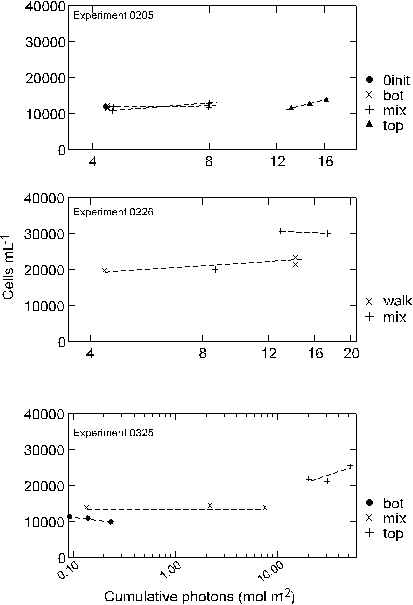
experiment 0205 MIX bottles traversed the light gradient twice,
once every 24 hours, and were sampled every 12 hours (Figure 9).
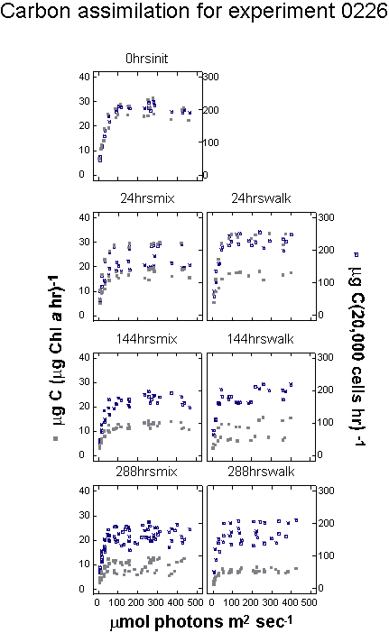
The entire experiment lasted 48 hours. In experiment 0226 samples
made the same number of gradient traversals as 0205, but it required
144 hours, or six days, for each traversal. Under these conditions,
the cells were exposed to six days of increasing light intensity
and had nearly an entire day at full intensity before descending
through a decreasing light gradient. Experiment 0325 used the same
mixing period as 0205, but added seven days of acclimation prior
to the first sampling and lasted 96 hours instead of 48.
Experiment 0205, with the shortest duration of all the experiments,
showed little change in the cell density over the 48 hours
(Figure 10). Cell counts ranged from 11,945 cells mL-1
at the start, to 13,781 cells mL-1 at 48 hours in the
TOP bottles where light was maintained at ~250 mmols
throughout the experiment. In comparing the influence of increasing
overall light availability, the un-mixed BOT, mixed and un-mixed
TOP samples increased cell density at the daily specific growth
rate of 0.02, 0.03 and 0.07, over the course of the experiment respectively
(Appendix A). A regression of cell density against cumulative
light exposure by treatment indicated that throughout the study
the 0205 and 0325 experiments were significantly correlated with
a treatment�s light exposure (Table 3, Figure 11).
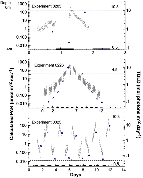
|
Figure
9.Photosynthetically
available radiation received by each treatment.
|
Photosynthetically
available radiation received by each treatment.
Recorded light
intensity for each mixed experiment (gray dots). The gray
dots
also generally
describe the position of the bottles in the column with lights
on.
Bars along the
X axis indicate 12 hour dark periods.The second vertical axis
describes the 24-hour
summation of light that each replicate bottle received
during an experiment.
This total daily light dose (TDLD) for the mixed
treatments is represented
by large dots. Solid dots indicate TDLD's at sampling
times and open
circles indicate TDLD's at times when no samples were taken.
The dashed horizontal
lines represent TDLD for the control bottles. The upper
lines are for the
TOP controls and the lower lines are for the BOT controls.
Experiment 0226
had a single set of controls left in the environmental chamber.
|
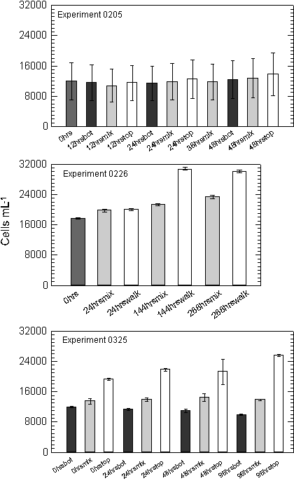
Cell
densities in the second experiment (0226), which ran for 288 hours,
ranged from 17,591 at the start of the experiment, to 30,010 after
288 hours in the walk-in chamber (0.04 specific growth rate).
The cell density in the mixed samples was 23,377 cells mL-1
at the conclusion of the experiment (0.02 specific growth
rate). A plot of cell density against cumulative light history for
the two treatments indicated that growth rate was much higher in
the chamber where both cumulative light and temperatures were higher
(Table 3, Figure 11).
Cells
in the third experiment, having spent seven days acclimating to
varied light climates showed a divergence in cell density between
treatments by the first day of sampling. No cell counts were taken
prior to the acclimation period. Following the acclimation period
cell densities in the BOT treatment, were 11,914 cells mL-1
and declined to 9,874 by the end of the experiment (-0.05 specific
growth rate). The BOT treatment showed decreased cell density each
sampling period over the entire 96-hour sampling period. Bottles
in the MIX treatment increased slightly from 13,494 to 13,836 during
the same four-day sampling period (0.01 specific growth rate). Cell
density in the fixed TOP treatment increased the greatest
from 19,274 to 25,551 cells per mL over the sampling period (0.07
specific growth rate).
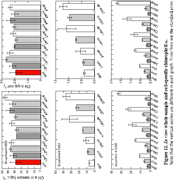
Whole sample chlorophyll a in the first experiment (0205)
was initially
38.7 mg L-1 at the start of the experiment (Figure 12 and Appendix
B). After 12 hours, chlorophyll increased in all treatments.
However, by 24 hours chlorophyll in the BOT and MIX treatments both
declined to 37.5 and 37.0 mg
L-1 respectively. Chlorophyll in the 24-hour TOP sample
declined from the 12-hour sample, but was still higher than the
starting value. By 48 hours, all samples had increased whole water
chlorophyll a over initial concentrations. When the whole
water chlorophyll concentrations were normalized on a per cell basis,
thereby providing an estimate of cellular pigment content, the trends
were the same over the course of the experiment. The initial pigment
content per cell was 1.9 pg cell-1, which increased to
2.3, 1.9 and 2.4 for the BOT, MIX and TOP treatments after 48 hours.
In
addition to chlorophyll a, chlorophyll c1+c2 and the
carotenoids fucoxanthin and b-carotene
were measured. Although the absolute concentrations of the carotenoids
could not be determined spectrophotometrically, their relative importance
to the in vitro pigment absorption was derived for their
associated absorption maximums.
For
the first experiment, fucoxanthin-like absorbance (FLA) and b-carotene-like absorbance (BLA) correlated strongly with each
other and with chlorophyll a only in the MIX samples (Appendix
C). TheTOP and BOT samples had strong correlation
between fucoxanthin
and b carotene only, and neither pigment correlated well
with chlorophyll
a.
Chlorophyll a in the whole samples for experiment 0226 increased
in a more predictable fashion, increasing in both the mixed and
stationary (WALK) treatments at every sampling period (Figure 13b).
The initial sample contained 7.0 mg
L-1 that increased slightly after 24 hours to 8.4 and
10.5 mg L-1 for
the MIX and WALK treatments respectively. After 144 hours the chlorophyll
a in the MIX treatment had doubled to 15.2 mg L-1 while the chlorophyll
a
in the WALK samples increased by a factor of 4.5 to 31.5 mg L-1. By 288 hours the MIX
samples
increased by another 8 mg
L-1 while the increases in the WALK samples slowed so
that only 4 mg L-1 was
accumulated over that
observed in the 144-hour samples. As in the first experiment, cellular
pigment contents followed the same temporal relationships as that
in the whole samples. This indicates that changes in whole
sample pigment concentrations were more influenced by population
growth than by cells synthesizing more pigment. The initial value
was 0.4 pg cell-1 which increased to 1.0 and 1.2 for
the MIX and WALK treatments after 288 hours. In the last 144 hours,
the MIX cells added 0.26 pg cell-1 chlorophyll a,
while the WALK cells added only 0.15. FLA and BLA correlated strongly
with each other and with chlorophyll a in the WALK treatment.
Though only the FLA:BLA correlated strongly in the mixed samples.
Chlorophyll a in experiment three (0325) followed a similar
trend as cell density in the same experiment, which was generally
to attain three very different concentrations by treatment before
the sampling phase began. Chlorophyll a increased steadily
in the TOP samples throughout the sampling period from 11.0 mg
L-1 at time zero and finishing at 32.86 mg
L-1 96 hours later. However, both the BOT and MIX treatments
lost chlorophyll a over the course of the experiment. Again,
the same trends were noticed in the cellular chlorophyll content
as in the whole sample chlorophyll. Samples in the TOP treatment
added cellular chlorophyll a (0.16 to 1.7 pg cell-1)
despite being continuously expose to irradiances of about 110 to
225 mmol throughout the
bottle cluster. Samples in the MIX and low light, BOT treatments
lost chlorophyll over the 96 hours. The final experiment indicated
strong correlation between fucoxanthin, b
carotene and chlorophyll in all treatments throughout the experiment.
Regression analysis of various pigments against TDLD
was conducted
to determine if particular pigment concentrations would be responsive
to a cell�s light history. Cellular estimates of chlorophyll a,
FLA, BLA, Pheo a and Chl c were regressed against
the daily light dose received by each treatment. The relationships
were significantly linear and positive for all pigments in the 0325
experiment. There were large differences in the number of replicates
for each experiment in the regression analysis. This makes the comparison
of significance between experiments difficult.
As
stated earlier, C assimilation across a range of irradiances was
parameterized for each replicate sample in two ways. The first used
a statistical software package to fit the points to a model that
included a term that describes the Y intercept of the fitted curve.
The points used in this statistical routine were whole sample C
assimilation values normalized to cell density in the sample. The
parameters derived from this method are hereafter referred to as
Pmax and a.
Scatter plots of the cell-specific photosynthesis (CELLC14)
versus irradiance curves allow visual interpretation of the relationships
between the treatments (Figure 13 a,b,c).
The
second method fitted the same replicates using a similar model and
a program developed specifically for determining photosynthesis
versus irradiance parameters (Fee 1998).
|
Figure
13 a, b and c. Photosynthesis versus irradiance plots.
|
|
Each curve represents
the photosynthesis versus irradiance relationship for each
replicate bottle in an experiment. Each square plot has two
curves for the same bottle. The gray points correspond to
carbon assimilation per unit chlorophyll a in the whole
sample (PB) and the dark points correspond
to assimilation normalized for cell density.
|
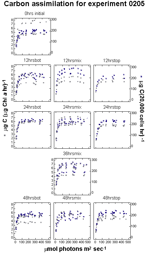
Figure 13b
Figure
13c
The
replicates of C assimilation values were then normalized to the
cell density in the sample and the mean concentration of chlorophyll
a per cell. The cell-specific parameters are referred to
as Pcellmax and acell, and the
cellular chlorophyll-specific
parameters are referred to as PBmax
and aB.
Pmax/a
and Pcellmax/acell describe the
same data,
but represent two methods of calculating the parameters with
Pmax
and a being calculated
with the Platt 1976 model with R and Pcellmax
and acell
calculated with the Fee
applications. PBmax/aB are not normalized to whole water chlorophyll
a, but rather to cellular chlorophyll a in pg
cell-1
(Bcell).
For
the parameters Pmax and a,
visual inspection and one-way ANOVA analysis indicated no difference
between any two temporally consecutive parameters from the same
treatment in the 48-hour experiment (0205) or the 288-hour experiment
(0226) (Table 3). That is, no coherent trend was seen in figure
14 in relation to daily light exposure (dots). The uncertainty in
the parameter estimates (described in the figure with bars showing
the 5% confidence intervals) indicate that the parameters did not
change statistically during the experiment. However, some
qualitative changes in the means are discernable.
Only
the 0325 experiment, which acclimated the diatom cultures to the
experimental light regime prior to any photosynthetic assays, showed
statistically significant change in photosynthetic parameters within
a single experiment. A one-way ANOVA categorically comparing
Pmax
and a with TDLDs as categories
determined that the third and fifth measurements of Pmax in experiment
0325 were significantly distinct from the other three MIX sample
periods at the 5% level (Table 2). A Tukey post hoc test
confirmed the significance and also showed that sample periods 4
and 5 (72 and 96 hours) are not statistically different from each
other, but were significantly different from 2 and 3 (24 and 48
hours). Samples 1,2 and 3 are not statistically separate values.
In
a scatter plot of the Pmax values for the individual
replicate MIX bottles versus TDLD, distinct clusters of points occur
only in the 0325 experiment (Figure 16). In the previous two
experiments,
there was no clear trend in the relationship between 24-hour light
history and maximum photosynthetic capacity. This relationship is
also seen in a multiplot of the treatment means of Pmax
and a plotted against the
TDLD (Figure 17). In this figure, the results from the practice
experiment 1212 are also shown. In experiment 1212 only static TOP
and BOT samples were incubated for two days at high and low light.
By the second day, Pmax and a had shifted very slightly from the
initial
reading.
Lack
of estimates of variance for the parameter estimates of
Pcellmax/acellmax and
PBmax/aB prevent statistical
comparisons
to verify whether two estimates are distinct. However, the values
did reveal interesting relationships (Figures 16,17). Neither
Pcellmax
nor PBmax for experiment 0205 varied throughout
the experiment and generally agrees with the lack of variation
Pmax
for 0205.
For
experiment 0226, aB
varied little for the chamber treatment where conditions were consistent
for the entire experiment. A slight decrease in aB
for the chamber during the experiment is not seen in the acell parameter, which
indicates
an increase in cellular chlorophyll with no change in a itself. In the MIX treatment, acell
increases slowly throughout the experiment, though aB declines sharply at 144 hours, along with an increase
in Bcell.
|
Figure
14a, b, and c. cell-specific photosynthetic parameters.
|
|
Photosynthetic
parameters calculated using the three-parameter model of
Jassby
and Platt (1976) with the R respiration and aggregated using
the stepwise method. Carbon assimilation is for 20,000 cells
hour-1. Error bars are the 5% confidence intervals
about the estimates. Total daily light dose (TDLD) calculated
as mmol photons
m-2
day-1 have been overlaid on the graphs to describe
the light history experienced by the cells in given treatment.
|
|
Figure
15 d, e, f. Cell-specific photosynthetic parameters.
|
|
Photosynthetic
parameters calculated using a two-parameter formulation of
the Jassby and Platt (1976) model without the R respiration
term (Fee, 1998). Carbon assimilation is corrected for
cell-density
per cell and is mg
14C per 20,000 cells.
|
Table
of Contents
The
definition of photoacclimation for this study is a clear
correlation
between the light history of a diatom species and the measure of
a variable indicative of their photophysiological status. This
study
was conducted to address the hypothesis that photoacclimation
occurs,
and can be detected, in algae that traverse a light gradient
that
ranged 200 mmol over a
period
of hours to days.
Common
parameters that can describe the physiological status of an
algal
population include maximum photosynthetic capacity
(Pmax)
and efficiency (a), and
chlorophyll-specific absorption cross-sections
(Anning et al. 2000; Falkowski and Owens 1980; Falkowski
and Raven 1997; Flameling and Kromkamp 1997; Vidussi et
al.
1999; Vincent et al. 1994). The original goals of the
project
were to detect and quantify photoacclimation in response to a
range
of mixing velocities that would move algal cells through a light
gradient at different rates. If possible, I hoped to determine
an
upper boundary of mixing rate, beyond which the rate of mixing
would
exceed the rate of acclimation and no difference in
photosynthetic
state would be discernable between cells taken at the top and
bottom
of the mixing cycle. Despite the slow rate of simulated
mixing
used throughout this study, photoacclimation was suggested in
two
experiments, and confirmed in only the final experiment.
Although
state transitions and non-photochemical quenching mechanisms in
the photosynthetic biochemical pathways can adjust
light-absorbing
cross-sections of cells on the order of minutes,
photoacclimation
is generally referred to as a longer-term process (Falkowski and
Raven 1997). They go on to cite others when they describe the
potential
for chlorophyll per cell or per unit surface area to increase
five-
to ten-fold as irradiance decreases (Falkowski and Owens 1980;
Prezelin
and Matlick 1980; Ramus 1990; Richardson et al. 1983).
However,
there are cellular chlorophyll minima that occur at both ends of
a continuum from low to high irradiances. At low irradiance, the
cells become chlorotic, or lacking color, and respond by
increasing
cellular chlorophyll a content until a maximum quota is
reached
at an intermediate irradiance. At irradiances that are higher
still,
cells respond by decreasing chlorophyll content and production
until
a minimum is reached. For example, an experiment using
Skeletonema
costatum and Dunaliella tertiolecta found that a
low
cellular chlorophyll content at an irradiance of 1-10 mmol
quanta m-2 sec-1 increased to a maximum at
~20 mmol quanta
m-2 sec-1.
With higher irradiance, a decline in cellular chlorophyll was
seen
until ~400 mmol quanta
m-2 sec-1 (Falkowski
and Owens 1980).
Contrary
to expectations chlorophyll increased more rapidly in the
high-light
WALK and TOP treatments than lower light treatments in each of
my
experiments. This suggests that cells may have been light
limited
and had not reached their maximum chlorophyll content.
However,
cellular chlorophyll in experiment 0205 did not increase
significantly
and began with initial replicates with cellular chlorophyll
already
just below 2.0 pg cell-1. This experiment also showed
the highest per cell chlorophyll concentration of the study with
a single treatment having an average 2.5 pg cell-1.
This
represents a cellular maximum for the conditions in this study.
The remaining treatments in experiment 0205 averaged around 2.0
pg cell-1. The TOP treatments in 0226 and 0325
experiments
increased cellular pigment from about 0.4 at the start of each
sampling
period to a maximum of about 1.5 pg by the time each experiment
ended. The continual increase in cellular chlorophyll a
in
the second two experiments is consistent with the assumption
above
that cell pigment maximums were about 2.5 pg.
The
lack of chlorophyll production in the BOT replicates of
experiment
0325, where light was ~10 mmol,
falls within expectation based upon the previous studies on
diatoms
described above. Similarly, the MIX samples which were often
below
50 mmol lost chlorophyll
in experiment 0325 and only gained chlorophyll after 24 hours in
experiment 0226 when the cells emerged from a long duration at
low
light.
Pigmentation
did not correlate with light history in any consistent way
except
that cells with exposure to high light approached cellular
chlorophyll
a maximums for this study. At the same time, the light
limited
bottom treatments appeared to be unable to synthesize more
pigment.
Variability in the pigmentation in each treatment was greatest
in
the top samples where the light gradient due to the position of
the bottles in relation to the attenuation of light was
steepest.
Simply due to the attenuation of light in the columns, bottles
at
the top of the TOP cluster experienced average irradiance of
about
225 mmol, while those at
the bottom of this cluster
received slightly over 110 mmol.
Shading by the bottles themselves may have further increased the
differential.
The
amount of chlorophyll a and the estimate of accessory
pigments
did not change relative to each other throughout the study. That
is, changes in pigmentation seemed to occur for all
photosynthetic
pigments in concert. Throughout the study, chlorophyll generally
correlated with FLA and BLA. However, in some cases the
relationships
were inexplicably negative or in some cases not correlated at
all.
No clear trend was seen in regards to treatment of light
exposure,
which would have also hinted at a chromatic response (Appendix
C).
The
qualitative changes in the light environment within the
experimental
columns were not quantified, however some information was gained
through simple observation. Light reaching the bottom of the
columns
was visible when clear plates of Plexiglass on the column
bottoms
were uncovered. By holding a white piece of paper underneath the
plates, the white light entering the columns at the top was blue
at the bottom. It was clear that the longer visible
wavelengths
had been filtered by the water in the columns. The scattering
and
refracting influence of the bubbles in the columns appeared to
mute
this selective filtering and the light became slightly more
white
when bubbles were present. Without a spectroradiometer there was
no way of knowing the exact spectral quality that reached the
bottom
of the columns. However, despite the bluing of the light, Morel
et al. 1987 determined that light intensity was of much greater
importance to photoacclimation than light quality in the diatom
Chaetoceros protuberans. (Morel
et al. 1987)
The
changes in light color with depth in the columns were apparent.
According to theories of chromatic acclimation, A.
Formosa
should have modified its pigment ratios to optimize its
photosynthetic
action spectra for the bluer light deep in the columns. Kirk
(1996)
summarizes numerous studies and taxa-specific responses when he
says that accessory pigments will often increase more rapidly
than
chlorophyll a in response to lowered light or shifted
spectra.
With fucoxanthin as the primary, photosynthetically coupled
accessory
pigment, any chromatic acclimation should have been detected
through
a ratio change with chlorophyll a. However, the lack of
consistent
shift in the concentration of pigments in relation to each other
might have indicated that the light gradient and the change in
quality
was not great enough for the cells to undergo chromatic
acclimation.
Although shifts in pigment ratios due to chromatic acclimation
are
common across algal groups, further studies cited by Kirk (1996)
seem to indicate that fucoxanthin is particularly stable when
faced
with shifts in light quality (Brown and Richardson 1968; Shimura
and Fujita 1975). This lack of plasticity in
fucoxanthin:chlorophyll
ratios agreed with results described previously in this study.
Detection
of a coherent pattern of acclimation in this study was
difficult.
The results from the cellular pigmentation and photosynthetic
parameters
indicate that changes in the cells held under control conditions
were occurring despite being held in an unchanging environment.
Comparison of the photosynthetic parameters
Pcellmax
and acell
describe
cell-specific acclimation regardless of the cellular chlorophyll
content. These parameters can describe the particular strategy
of
acclimation by the plankton. Photosynthesis versus irradiance
relationships
will tend to change with changes in size or number of
photosynthetic
units (PSUs).
Increasing
number or size of PSUs each represents a different strategy for
photoacclimation and was thought to be taxa specific. However,
conflicting
reports have prevented simple taxonomic-based classifications
(Falkowski
and La Roche 1991). Recently, some authors have proposed that
the
nature of the photosynthetic response is more due to the peak
intensity
received by the cells or the total light dose (Ibelings et
al.
1994; Kromkamp and Limbeek 1993; Kroon et al. 1992b). In
a simple visualization of Pmax versus TDLD for the
MIX
treatment replicates, only the 0325 experiment showed a positive
relationship between the maximal photosynthetic rate and the
overall
light exposure (Figure 16).
If
the size of the PSU is increased, acell
will increase due to an increase in the number of light
harvesting
pigment molecules. However, Pcellmax will
not change because additional reactions centers are not added.
If
Pcellmax increases, it is due to the
synthesis
of more PSUs or reactions centers. The addition of reaction
centers
and PSUs will also raise acell because they contain chlorophyll a (Falkowski
and La Roche 1991; Lewis et al. 1984a).
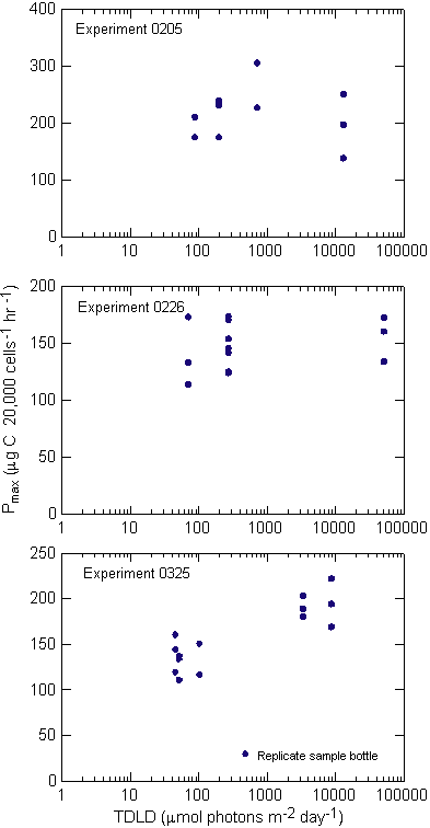
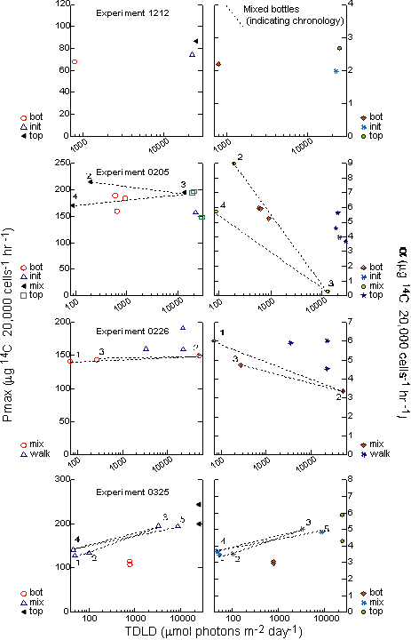
Use
of chlorophyll as the normalization factor describes the
efficiency
of photosynthesis, whereas simply normalizing photosynthesis
per
cell provides a measure of how effective a cell is at
assimilating
carbon.
It is important to remember that the
TOP
and BOT controls in the first experiment provide secondary
results
that describe a situation as found in studies such Anning
et
al. (2000). Those experiments were conducted using
abrupt changes
in light intensity to study acclimation. The same changes
were included
in this experiment as well as the oscillating MIX treatment.
Because
the cells were initially grown at ~100 mmols
(INIT) and placed directly into the BOT treatment at ~10
mmols
or the TOP treatment at ~250 mmols, these treatments may be used as
time series test to
determine when a steady state is reached after a shift to a
new
light intensity.
In the BOT treatment, acell continued to
climb at a rate of about 2 mg C (20,000
cells)-1 mmol photons�1 m-2
per day over the entire
experiment and never came to a complete steady state (Figure
15
D). The increase in photosynthetic efficiency in the BOT
cells may
have been reflected in the Bcell values as they
increased
from 1.9 pg chl a cell-1 in the INIT
replicates
to 2.0 at 24 hours then to 2.3 at 48 hours (Appendix F). The
sample
taken after 12 hours showed a value of 2.2, but this may
have been
due to diel effects and cell cycle differences between the
other
two samples. The influence of diel effects within each
experiment
were removed because each sample was taken at 24 hour
intervals,
except for 0205 where samples were taken at 12 hours
intervals as
well. Because acell increased steadily and
Pcellmax decline
steadily, Ikcell also declined over
the experiment
in a response cited in most static photoacclimation studies.
Unfortunately,
the TOP and MIX treatments in 0205 did not have a consistent
response
to their new light climate.
In
a study of Skeletonema costatum, Kromkamp and Limbeek
(1993)
determined that during acclimation to a fluctuating light
climate
(PAR oscillations every two hours at 17 � C), the diatom S.
costatum decreased
photosynthetic unit (PSU) size and increased the number of
PSUs.
They also found that when the peak PAR exposure throughout the
cycle
was 167 mmol
m-2 sec-2 (at ~30
mmol, TDLD=0.86 mol
day-1), the photoacclimation
response was muted when compared to similar treatments which
oscillated
from 100 �320 mmol
m-2
sec-1 (TDLD=1.72 mol day-1). Because
this
study did not consider chlorophyll-specific photosynthetic
cross-sections,
I cannot describe with certainty the strategy of
photoacclimation
employed by A. formosa. However, cell-specific
photosynthesis
parameters, modeled using the Fee application, suggest that
A.
formosa both increased the number and size of PSUs when
adjusting
to low light in all experiments (Figure 15).
Diatoms
as a group are tolerant of cool to cold temperatures within
the
range of those used in this study. As evidence of this,
measurements
taken in Antarctic freshwaters at 0 to 4 �
C reveal estimates of photosynthetic rates similar to, or
greater
than, temperate or tropical waters (Hawes 1990). Butterwick et
al.
studied the implications of temperature on growth rates for
several
species of freshwater phytoplankton. Under a constant light of
100
mmol, Asterionella
formosa
and seven other species were grown at temperatures from 2
� to 35 �
C. A. formosa had a peak growth rate of 1.68 divisions
day
�1 at 20 �
C
and was the most tolerant of low temperatures with a growth
rate
of 0.61 divisions day �1 at 5 � C (Butterwick et
al. 1987). Kozitskaya
(1992) conducted a similar study with four marine species
including
the diatoms Phaeodactylum
tricornutum
and Navicula atomus at
temperatures
of 10 �, 20 �
and 30 � C. She found
that
at 10 � C both species
had average growth rates over
the course of 20-25 days, of 0.059 and 0.110 divisions day
�1
for P. tricornutum and N. atomus respectively.
She
also found that as a rule, diatoms in her study preferred
temperature
at or below 15 � C.
Cold
temperatures appear to have the effect of prematurely inducing
photoinhibition
and excessive photoexcitation in cells as they are brought
into
high light from low light (Falkowski and Raven 1997; Platt
et
al. 1980). The primary cause for this is that the rate
of photon
capture is largely temperature independent, as indicated by
the
lack of sensitivity of light-limited photosynthetic efficiency
(a)
to changes in temperature. However, the rate of
enzyme-mediated
electron transport is temperature sensitive and the maximum
rate
of photosynthesis (Pmax) will decline with
decreasing
temperature. Therefore, reduced temperatures allow for the
same
rate of photon capture, but a reduced ability to process
potentially
damaging excessive photo excitation. This effect is further
aggravated
when cells are shade-adapted and their photon-capturing
�antennae�
are fully exposed.
For
these reasons, the potential for a photoprotective response by
the
cells seemed possible. However, there were no unusual
increases
b-carotene throughout the study that would have indicated a photoprotective
response. However, I was unable to measure the other
xanthophyll
photoprotectants, which could have increased when the
low-light
acclimated cells were brought into the high light present
particularly
at the top of the columns.
Thompson
et al. (1992) in a study of the effects of temperature
on
eight species of marine phytoplankton found that chlorophyll
a
per cell was always lower at 10 �
C than at 25 � C, for
the same light intensities. Similarly,
the carbon:chlorophyll a ratios increased with
increasing
temperatures for all species, suggesting a
temperature-mediated
partitioning of resources. The cold conditions likely hampered
the
cells� abilities to photoacclimate under all light
environments.
Cells that are limited by temperature and light had the least
ability
to photoacclimate, despite the fact that the media was replete
with
nutrients. At the end of experiment 0205 dissolved phosphorus
was
still above 8.2 mmol
L-1
after beginning the experiment at 8.5 mmol
L-1. Phosphorus does not become limiting until well
below
1 mmol L-1.
Dissolved silica, the next
likely limiting nutrient, was not measured (Kilham and Tilman
1976).
Most
prior studies have considered photoacclimation under
conditions
that were 15 � C or
warmer (Anning et al. 2000; Cullen
and Lewis 1988; Falkowski 1980; Falkowski 1984a; Geider et
al.
1986; Grobbelaar et al. 1995; Grobbelaar et al.
1996;
Ibelings et al. 1994; Marra 1978). There is strong
experimental
evidence that Pmax strongly correlates with temperature,
though
a does not
consistently
do so (Coles and Jones 2000; Jones 1998; Keller 1988). This
appears
to be true in this study where Pcellmax
remained
constant in the replicates that were left in the environmental
chamber
(WALK), while bottles that were placed in the columns that
were
11 � C colder showed
depressed, but largely invariant
Pcellmaxs over the experiment. In the
same
experiment, acell
actually increased in both treatments, which was expected for
the
MIX bottles, but not those left in the constant conditions of
the
chamber.
Only
after a ten day entrainment in the oscillating irradiance did
photoacclimation
become significance enough to confirm. These results suggest
the
possibility that under poorly lit and cold conditions, diatom
photoacclimation
occurs more slowly than indicated by previous studies
conducted
under warmer and brighter conditions. The reduction in
available
light energy and suppression of biosynthesis by sub-optimal
temperatures
appeared to reduce the ability of A. Formosa tooptimize
its
photophysiology to match its slow traversal of a light
gradient.
Others
have suggested the potential for phytoplankton to become
accustomed
to regular light fluctuations overlaid with normal diel
patterns
(Prezelin and Matlick 1980; Prezelin and Sweeney 1977). That
ability
would explain the results found in the final experiment. Such
a
complex adaptability to a fluid environment that is known for
being
highly turbulent and irregular seems unlikely. Turbulence at
the
scale of Langmuir circulations or smaller likely present
highly
variable oscillations of the light environment to the
entrained
plankton.
Although
complete darkness was not achieved at the bottom of the
columns,
the cells were unable to gather enough light to synthesize
significant
quantities of pigment, improve their photosynthetic efficiency
or
increase in number. This light level, which proved
insufficient
to support cell growth, approximates that observed at 16.5
meters
at the Fox Point station during the spring (Figure 18).
A.
formosas� ability to photosynthesize at low irradiances
seemed
to be impacted by their low chlorophyll, as
Pcellmax
and acell were slow
to increase during
experiment 0325 and followed cell chlorophyll content. Low
chlorophyll
and the requirement for sufficient photon capturing ability to
synthesize
more represent a negative compounding effect. For example, the
BOT
samples in this study were shown to be unable to synthesize
photopigments,
perhaps due to light limitations. This suggests that
photoacclimation
at depths near 16.5m, or deeper, would be hampered or even
cease
if cells remained at such low intensities for a week or
longer.
That is, the compensation depth would be shallower than 16.5
m.
Experiment
0325 indicates that cells would have the ability to acclimate
if
they were entrained in turbulence circulation near the surface
for
long periods. However, due to their severe light stress, cells
that
spent long periods in darker conditions would suffer a lag in
their
ability to rapidly acclimate to higher light. This may account
for
descriptions of hystersis in the literature (Cullen and Lewis
1988).
It also might mean that in profiles of algal cells and
chlorophyll
in Lake Michigan, cells that were taken from consistently dark
depths
(<10 mmols) and are
found
to be deficient in chlorophyll a, likely have spent
seven
days or more at or below that depth. My study suggests that
cells
that are mixed to greater depths must get to the surface often
enough
to capture sufficient light to conduct biosynthesis and hence
photoacclimate.
This
study did not detect strong photoacclimation in samples that
were
immediately introduced into an oscillating light regime after
an
extended period under static lighting. Some results indicated
that
photoacclimation was occurring in the samples that were passed
through
a very slowly oscillating light environment. However,
that
acclimation did not result in the modulation of cellular
pigment
content. Instead, changes in the �package effect� of the
photosynthetic
apparatus in the cells likely accounted for the adjustments in
photosynthetic
capacity.
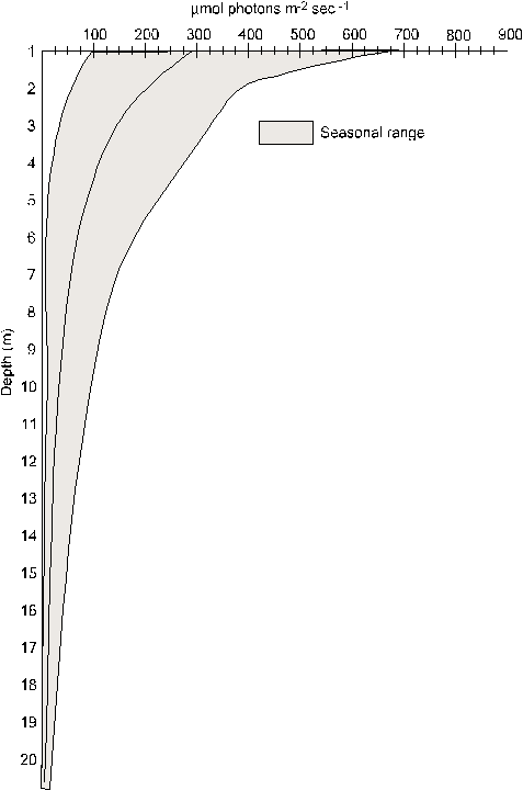
The
relationship between Ikcell and the
total
daily light dose is a classical one that agrees with
expectations.
The offset of the data points from the WALK treatment in
figure
19 may be because they were much warmer than the rest of
the treatments
at 4 � C.
Unfortunately,
the trend should have raise Ik values above the
colder
treatments, not decreased it. As the cells are exposed to
greater
and greater amounts of light, their maximal photosynthetic
rates
increase to make use of the added light. As the depth of
mixing
shoals and seasonal light intensity increases in the
spring, the
community photosynthetic status should move from left to
right in
figure 19, and degrade in the fall.
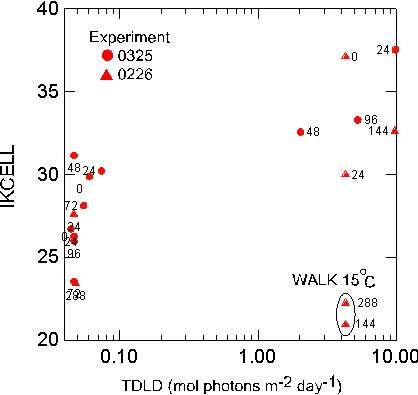
Table
of Contents
Conclusion
Asterionella
formosa used both increases in the number and size
of photosynthetic
units to acclimate to lower irradiances. These increases
occurred
within 24 hours of being introduced into a new light
climate, though
clear trends in the response of photosynthetic parameters
and pigments
to light history was tenuous in two of three experiments.
In general,
the photoacclimation response included synthesis of
photosynthetic
pigments that appeared to be proportional to each other
across all
light histories and maximal intensities. This
proportionality in
pigmentation included samples taken from the darker and
bluer BOT
treatments, where the potential for chromatic adaptation
to alter
pigment ratios was highest. However, after one week the
cells in
the BOT treatment became so light limited that they were
incapable
of synthesizing pigment and the cell density began to
decline. This
indicates that cells require certain total light dose in
order to
successfully photoacclimate to dark conditions.
Contrary
to published trends, the TOP samples in all experiments
increased
or maintained chlorophyll content despite being in light
that should
not be limiting. Unless the light at the top was indeed
sub-saturating
to the cells. It appeared that the cells needed to add
chlorophyll
until they approached a maximum of about 2.5 pg
cell-1,
where cells in experiment 0205 seemed to maintain their
content.
The final experiment yielded the most consistent evidence
of periodic
photoacclimation that was correlated with daily light
history. The
fact that this periodic acclimation only became apparent
after ten
days under the mixed light regime suggests that
acclimation to a
non-diel, cyclic light cycle may be occurring.
Anning,
T., H. L. MacIntyre, S. M. Pratt, P. J. Sammes, S. Gibb
and R. J.
Geider (2000). �Photoacclimation in the marine diatom
Skeletonema
costatum.� Limnology and Oceanography
45(8): 1807-1817.
Arar,
E. J. (1997). Method 446.0: In vitro determination of
chlorophylls
a, b, c1 + c2 and pheopigments in marine and freshwater
algae by
visible spectrophotometry. Cincinnati, OH 45268,
National Exposure
Research Laboratory, Office of Research and Development,
U.S. Environmental
Protection Agency: 1-26.
Berner,
T., Z. Dubinsky, K. Wyman and P. G. Falkowski (1989).
�Photoadaptation
and the "package effect" in Dunaliella
tertiolecta
(Chlorophyceae).� J. Phycol. 25(70-78).
Brooks,
A. S. and D. N. Edgington (1994). �Biogeochemical
Control of Phosphorus
Cycling and Primary Production in Lake-Michigan.�
Limnology and
Oceanography 39(4): 961-968.
Brown,
T. E. and F. L. Richardson (1968). �The effect of growth
environment
on the physiology of algae: light intensity.� J.
Phycol.
4: 38-54.
Butterwick,
C., S. I. Heaney and J. F. Talling (1987). �The
Influence of Temperature
on Algal Growth.� British Phycological Journal
22(3):
301-301.
Coles,
J. F. and R. C. Jones (2000). �Effect of temperature on
photosynthesis-light
response and growth of four phytoplankton species
isolated from
a tidal freshwater river.� Journal of Phycology
36(1):
7-16.
Cuhel,
R. L., D. Ortner and R. S. Lean (1984). �Night synthesis
of protein
by algae.� Limnol. Oceanogr. 29(4):
731-744.
Cullen,
J. J. and M. R. Lewis (1988). �The kinetics of algal
photoadaptation
in the context of vertical mixing.� J. Plankton
Res. 10(5):
1039-1063.
Dubinsky,
Z., P. G. Falkowski and K. Wyman (1986). �Light
harvesting and utilization
by phytoplankton.� Plant Cell Physiology
27: 1335-1349.
Dusenberry,
J. A. (2000). �Steady-state single cell model
simulations of photoacclimation
in a vertically mixed layer: implications for biological
tracer
studies and primary productivity.� Journal of Marine
Systems
24(3-4): 201-220.
Eilers,
P. H. C. and J. C. H. Peeters (1988). �A Model for the
Relationship
between Light-Intensity and the Rate of Photosynthesis
in Phytoplankton.�
Ecological Modelling 42(3-4): 199-215.
Fahnenstiel,
G. L., J. F. Chandler, H. J. Carrick and D. Scavia
(1989). �Photosynthetic
characteristics of phytoplankton communities in Lakes
Huron and
Michigan: P-I parameters and end-products.� Journal
of Great
Lakes Research 15(3): 394-407.
Falkowski,
P. G. (1980). Light shade adaptation in marine
phytoplankton.
New York, NY, Plenum Press.
Falkowski,
P. G. (1983). �Light-shade adaptation and vertical
mixing of marine
phytoplankton: A comparative field study.� J. Marine
Res.
41: 215-237.
Falkowski,
P. G. (1984a). �Kinetics of adaption to irradiance in
Dunaliella
tertiolecta.� Photosynthetica 18:
62-68.
Falkowski,
P. G. (1984b). �Physiological responses of phytoplankton
to natural
light regimes.� J. Plankton Res. 6(6):
295-307.
Falkowski,
P. G., Z. Dubinsky and K. Wyman (1985).
�Growth-irradiance relationships
in marine phytoplankton.� Limnol. Oceanogr.
30(2):
311-321.
Falkowski,
P. G. and J. La Roche (1991). �Acclimation to spectral
irradiance
in algae.� J. Phycol.
Falkowski,
P. G. and T. G. Owens (1980). �Light-shade adaptation:
two strategies
in marine phytoplankton.� Plant Physiology
66: 592-595.
Falkowski,
P. G. and J. Raven (1997). Aquatic
photosynthesis. Malden,
MA, Blackwell Science, Inc.
Falkowski,
P. G. and C. D. Wirick (1981). �A simulation model of
the effects
of vertcal mixing on primary productivity.� Mar.
Biol. 65:
69-75.
Farmer,
D., J. Gemmrich and V. Polonichko (1998). Velocity,
temperature
and spatial structure of Langmuir circulation.
Physical Processes
in Lakes and Oceans. J. Imberger. Washington, D.
C., American
Geophysical Union. 54: 87-100.
Fee,
E. J. (1998). �Revision of: Computer programs for
calculating in
situ phytoplankton photosynthesis.� Can. Tech. Rept.
Fisheries
and Aquatic Sci. 1740.
Flameling,
I. A. and J. Kromkamp (1997). �Photoacclimation of
Scenedesmus
protuberans (Chlorophyceae) to fluctuating
irradiances simulating
vertical mixing.� Journal of Plankton Research
19(8):
1011-1024.
Gallegos,
C. L. and T. Platt (1982). �Phytoplankton production and
water motion
in surface mixed layers.� Deep-Sea Research
29(1a):
65-76.
Geider,
R. J., B. A. Osborne and J. A. Raven (1986). �Growth
photosynthesis
and maintenance metabolic cost in the diatom
Phaeodactylum tricornutum
at very low levels.� J. Phycol. 22: 39-48.
Goericke,
R. and N. A. Welschmeyer (1992). �Pigment turnover in
Thalassiosira
weisflogii. II. The 14CO2 labelling kinetics of
carotenoids
in a marine diatom.� J. Phycol. 28:
507-517.
Grobbelaar,
J. U., B. M. A. Kroon, T. Burgerwiersma and L. R. Mur
(1992). �Influence
of Medium Frequency Light Dark Cycles of Equal Duration
on the Photosynthesis
and Respiration of Chlorella- Pyrenoidosa.�
Hydrobiologia
238: 53-62.
Grobbelaar,
J. U., L. Nedbal, L. Tichy and I. Setlik (1995).
�Variation in Some
Photosynthetic Characteristics of Microalgae Cultured in
Outdoor
Thin-Layered Sloping Reactors.� Journal of Applied
Phycology
7(2): 175-184.
Grobbelaar,
J. U., L. Nedbal and V. Tichy (1996). �Influence of high
frequency
light/dark fluctuations on photosynthetic
characteristics of microalgae
photoacclimated to different light intensities and
implications
for mass algal cultivation.� Journal of Applied
Phycology
8(4-5): 335-343.
Harding,
L. W. J., B. W. Meeson, B. B. Prezelin and B. M. Sweeney
(1981).
�Diel periodicity of photosynthsis in marine
phytoplankton.� Mar.
Biol. 61: 95-105.
Harding,
L. W. J., B. B. Prezelin, B. M. Sweeney and J. L. Cox
(1982). �Primary
production as influenced by diel periodicity of
phytoplankton photosynthesis.�
Mar. Biol. 67: 179-186.
Hawes,
I. (1990). �The effects of light and temperature on
photosynthate
in Antarctic freshwater phytoplankton.� Journal of
plankton research
12(3): 513.
Ibelings,
B. W., B. M. A. Kroon and L. R. Mur (1994). �Acclimation
of photosystem
II in a cyanobacterium and an eukaryotic green-alga to
high and
fluctuating photosynthetic photon flux densities,
simulating light
regimes induced by mixing in lakes.� New Phytol.
128:
407-424.
Jeffrey,
S. W., R. F. C. Mantoura and S. W. Wright (1997).
Phytoplankton
pigments in oceanography. Paris, United Nations
Educational,
Scientific and Cultural Organization.
Jones,
R. C. (1998). �Seasonal and spatial patterns in
phytoplankton photosynthetic
parameters in a tidal freshwater river.�
Hydrobiologia 364:
199-208.
Keller,
A. A. (1988). �Estimating Phytoplankton Productivity
from Light
Availability and Biomass in the Merl Mesocosms and
Narragansett
Bay.� Marine Ecology-Progress Series
45(1-2): 159-168.
Kilham,
P. and D. Tilman (1976). �Some biological effects of
atmospheric
inputs to lakes: Nutrient ratios and competitive
interactions between
phytoplankton.� J. Great Lakes Res.
2(Suppli. 1):
187-191.
Kirk,
J. T. O. (1996). Light and Photosynthesis in Aquatic
Ecosystems.
New York, Cambridge Univ. Press.
Kromkamp,
J. and M. Limbeek (1993). �Effect of short-term
variation in irradiance
on light harvesting and photosynthesis of the marine
diatom Skeletonema
costatum: a laboratory study simulating vertical
mixing.� J.
Gen. Microbiol. 139: 2277-2284.
Kroon,
B. M. A., M. Latasa, B. W. Ibelings and L. R. Mur
(1992a). �An algal
cyclostat with computer controlled light regime.�
Hydrobiologia
238: 63-71.
Kroon,
B. M. A., M. Latasa, B. W. Ibelings and L. R. Mur
(1992b). �The
effect of dynamic light regimes on Chlorella. I.
Pigments and cross-sections.�
Hydrobiologia 238: 71-79.
Langdon,
C. (1987). �On the causes of interspecific differences
in the growth-irradiance
relationship for phytoplankton. Part I. A comparative
study of the
growth-irradiance relationship of three marine
phytoplankton species:
Skeletonema costatum, Olithodiscus leuteus
and Gonyaulax
tamarensis.� J. Plankton Res. 9:
459-482.
Laws,
E. a. and T. T. Bannister (1980). �Nutrient and light
limited growth
of Thalassiosira fluviatilis in continuous
culture, with
implications for phytoplankton growth in the ocean.�
Limnol.
Oceanogr. 25: 457-73.
Lehman,
J. T. (1976). �Ecological and nutritional studies on
Dinobryon Ehrenb.:
seasonal periodicity and the phosphate toxicity
problem.� Limnol.
Oceanogr. 21: 646-658.
Lewis,
M. R., J. J. Cullen and T. Platt (1984a). �Relationships
between
vertical mixing and photoadaptation of phytoplankton:
similarity
criteria.� Mar. Ecol. Prog. Ser. 15:
141-149.
Lewis,
M. R., E. P. W. Horne, J. J. Cullen, N. S. Oakey and T.
Platt (1984b).
�Turbulent motions may control phytoplankton
photosynthesis in the
upper ocean.� Nature 311(5981): 49-50.
Lewis,
M. R. and J. C. Smith (1983). �A small volume, short
incubation
time method for the measurement of photosynthesis as a
function
of incident irradiance.� Mar. Ecol. Prog. Ser.
13:
99-102.
Li,
M. and C. Garrett (1998). Large eddies in the surface
mixed layer
and their effects on mixing, dispersion and biological
cycling.
Physical Processes in Oceans and Lakes. J.
Imberger. Washington,
D.C., American Geophysical Union. 54: 61-86.
Lohr,
M. and C. Wilhelm (1999). �Algae displaying the
diadinoxanthin cycle
also possess the violaxanthin cycle.� Proc. Natl.
Acad. Sci.
USA. 96: 8784-8789.
Lorenzen,
C. J. (1967). �Determination of chlorophyll and
pheo-pigments: spectrophotometric
equations.� Limnol. Oceanogr. 12: 343-346.
Mac
Caull, W. A. and T. Platt (1977). �Diel variations in
the photosynthetic
parameters of coastal marine phytoplankton.� Limnol.
Oceanogr.
22: 723-731.
Mantoura,
R. F. C. and C. A. Llewellyn (1983). �The rapid
determination of
algal chlorophyll and carotenoid pigments and their
breakdown products
in natural waters by reverse-phase high performance
liquid chromatography.�
Anal. Chim. Acta. 151: 297-314.
Margalef,
R. (1958). Temporal succession and spatial heterogeneity
in phytoplankton.
Perspectives in Marine Biology. Berkeley, CA,
University
of California Press: 323-349.
Marra,
J. (1978). �Phytoplankton photosynthetic response to
vertical movement
in a mixed layer.� Mar. Biol. 46: 203-208.
Marra,
J. (1980). Vertical mixing and primary production.
In: Primary
productivity in the sea, P. G. Falkowski. New
York, Plenum Press:
531.
Morel,
A., L. Lazzara and J. Gostan (1987). �Growth rate and
quantum yield
time response for a diatom to changing irradiances
(energy and color).�
Limnol. Oceanogr. 32(5): 1066-1084.
Neale,
P. J. and P. J. Richerson (1987). �Photoinhibition and
the Diurnal-Variation
of Phytoplankton Photosynthesis .1. Development of a
Photosynthesis-Irradiance
Model from Studies of Insitu Responses.� Journal of
Plankton
Research 9(1): 167-193.
Perry,
M., M. Talbot and R. S. Alberte (1981). �Photoadaptation
in marine
phytoplankton: response of the photosynthetic unit.�
Mar. Biol.
62: 91-101.
Platt,
T., D. F. Bird and S. Sathyendranath (1991). �Critical
Depth and
Marine Primary Production.� Proceedings of the Royal
Society
of London Series B-Biological Sciences
246(1317): 205-217.
Platt,
T., C. L. Gallegos and W. G. Harrison (1980).
�Photoinhibition of
photosynthesis in natural assemblages of marine
phytoplankton.�
Journal of Marine Research 38: 687-701.
Platt,
T. and A. D. Jassby (1976). �The relationship between
photosynthesis
and light for natural assemblages of coastal marine
phytoplankton.�
J. Phycol. 12: 421-430.
Post,
A. F., Z. Dubinsky, K. Wyman and P. G. Falkowski (1984).
�Kinetics
of light-intensity adaptation in a marine planktonic
diatom.� Mar.
Biol. 83(231-238).
Prezelin,
B. B. (1992). �Diel Periodicity in Phytoplankton
Productivity.�
Hydrobiologia 238: 1-35.
Prezelin,
B. B. and R. S. Alberte (1978). �Photosynthetic
charateristics and
organization of chlorophyll in marine dinoflagellates.�
Proc.
Nat. Acad. Sci. 75: 1801-1804.
Prezelin,
B. B. and H. A. Matlick (1980). �Time-course of
photoadaptation
in the photosynthesis-irradiance relationship of a
dinoflagellate
exhibiting photosynthetic periodicity.� Marine
Biology 58:
85-96.
Prezelin,
B. B. and B. M. Sweeney (1977). �Characterization of
photosynthetic
rhythms in marine dinoflagellates. II.
Photosynthesis-irradiance
curves and in vivo chlorophyll a
fluorescence.� Plant
Physiology 60: 388-392.
Ramus,
J. (1990). �A Form-Function Analysis of Photon Capture
for Seaweeds.�
Hydrobiologia 204: 65-71.
Reynolds,
C. S. (1998). Plants in motion: Physical - biological
interaction
in the plankton. Physical Processes in Lakes and
Oceans.
J. Imberger. Washington, D. C., American Geophysical
Union. 54:
535-560.
Richardson,
K., J. Beardall and J. A. Raven (1983). �Adaptation of
unicellular
algae to irradiance: an analysis of strategies.� New
Phytol.
93: 157-171.
Rowan,
K. S. (1989). Photosynthetic Pigments of Algae.
New York,
NY, Press Syndicate - University of Cambridge.
Shimura,
K. and Y. Fujita (1975). �Changes in the activity of
fucoxanthin-excited
photosynthesis in the marine diatom Phaeodactylum
tricornutum
grown under different culture conditons.� Mar.
Biol. 33:
185-194.
Sukenik,
A., J. Bennett and P. G. Falkowski (1987). �The
Molecular-Basis
of Photoadaptation in the Marine Chlorophyte
Dunaliella-Tertiolecta.�
Israel Journal of Botany 36(1): 50-50.
Sukenik,
A., J. Bennett, A. Mortainbertrand and P. G. Falkowski
(1990). �Adaptation
of the Photosynthetic Apparatus to Irradiance in
Dunaliella-Tertiolecta
- a Kinetic-Study.� Plant Physiology
92(4): 891-898.
Sverdrup,
H. U. (1953). �On conditions for vernal blooming of
phytoplankton.�
J. Cons. Perm. int. Explor. Mer. 18:
287-295.
Vidussi,
F., J. C. Marty and J. Chiaverini (1999). �Phytoplankton
pigment
variations during the transition from spring bloom to
oligotrophy
in the northwestern Mediterranean sea - separation of
chlorophyll
a from divinyl-chlorophyll a and zeaxanthin from
lutein.� Deep
Sea Research Part I: Oceanographic Research Papers
47(3):
423-445(23).
Vincent,
W. F., N. Bertrand and J. J. Frenette (1994).
�Photoadaptation to
Intermittent Light across to St-Lawrence Estuary
Fresh-Water-Saltwater
Transition Zone.� Marine Ecology-Progress Series
110(2-3):
283-292.
Yoder,
J. A. and S. S. Bishop (1985). �Effects of
mixing-induced irradiance
fluctuations on photosynthesis of natural assemblages of
coastal
phytoplankton.� Mar. Biol. 90: 87-93.
Table
of Contents
Appendix
Appendix
G.DYV
Freshwater
Phytoplankton Medium
as modified
by Craig
Sandgren after
Lehman
1976, Limnol.
Oceanogr.
|
Reagent
|
DYV
amount
|
Final
Medium Concentration
|
|
Calcium
chloride (CaCl2)
|
0.8
g
|
180
mM
Ca
|
|
Magnesium
sulfate
(Mg(SO4)2 *
7H2O)
|
2.96
g
|
300
uM Mg
|
|
Sodium
nitrate (NaNO3)
|
0.8
g
|
235
mM
NO3-N
|
|
Ammonium
nitrate
(NH4NO3)
|
0.4
g
|
125
mM
NO3
& 125 mM
NH4-N
|
|
Potassium
chloride (KCl)
|
0.4
g
|
134
mM
K
|
|
Sodium
bicarbonate (NaHCO3)
|
0.8
g
|
250
mM
C
|
|
MOPS
buffer (pH 6.8)
|
10
g
|
|
|
Sodium
phosphate
(Na2HPO4)
|
0.262
g
|
46.1
mM
PO4-P
|
|
Sodium
metasilicate
(Na2SiO3
�
9 H2O)
|
0.6
g
|
53.2
mM
Si
|
|
DYV
vitamin working solution *
|
400
mL
|
|
|
DYV
micrometals working solution *
|
400
mL
|
|
For the WC
working
solution, add the WC metals �A� to 10
ml of super stock �B� &
then dilute to 1000 ml.
|
Table
3: WC micrometals
|
|
|
|
WC
dry metals �A�
|
|
|
|
EDTA
(Na2EDTA)
|
0.44
g/L
|
11.8
mM
EDTA
|
|
Boric
acid (H3BO3)
|
0.10g/L
|
17.7
mM
B
|
|
Ferric
chloride (FeCl3 *
7H2O)
|
0.10
g/L
|
3.7
mM
Fe
|
|
WC
metals super stock �B�
into 1 L
|
|
|
|
Zinc
sulfate (ZnSO4)
|
0.22
g/L
|
75
nM Zn
|
|
Cobalt
chloride (CoCl2 *
6H2O)
|
0.10
g/L
|
42
nM Co
|
|
Manganese
chloride (MnCl2 *
4H2O)
|
1.8
g/L
|
909
nM Mn
|
|
Sodium
molybdate
(Na2MoO4)
|
0.06
g/L
|
26
nM Mo
|
The vitamin
working
stock solution is a 1:100 dilution of
the following super stock
concentrate.
|
Vitamin
Mix Super Stock
|
|
|
|
Biotin
|
50
mg/L
|
5
mg/L
|
|
Thiamine
|
2000
mg/L
|
200
mg/L
|
|
Cyancobalamine
|
50
mg/L
|
5
mg/L
|
To make 2 L of
media
stock suitable for diluting to 40 liters
media. Dissolve the MOPS
buffer into 985 mL DDH2O. Correct to pH
6.8 with about 10 pellets
of NaOH and fine tune with 1 N HCl.
Weigh each reagent from Table
1 and add, in the order listed, to the
buffer solution while stirring
continuously. Add the working solutions
and dilute to 2 L. Store
in refrigerator; stable
indefinitely. To make the media,
add
50 mL of the media stock to 950 mL DDH2O
for each liter of media.
Autoclave or filter sterilize prior to
use.
As
modified from Dr.
Craig Sandgren�s
laboratory manual
using guidance from Lori Schaht
For use with
cultures
of densities 8500 cells/mL or greater
Radioactive
stock: NaH14CO3
(100 mCi/mL)
found in Radioactive Jeff�s
refrigerator
�Samples�
describes below
will yield one PvI curve of nine
points; one block can hold three
samples.
Scintillation cocktail
used at this time is Universol ES
Preparation:
Pre measure
sample (110
mL for #4) which will leave ~10 mL
when fully dispensed.
a.
Verify that
all lights in the block are working.
Light measurements should be
up to date for each well.
b.
Fill ice bath with
ice and start circulating pumps.
c.
Set working
temperatures on thermostat and wait
for blocks to cool to desired
temperature.
d.
Keep samples cooled
and room lights off.
e.
Put reagent
acid into plastic beaker for
pipetting.
Incubation:
1.
For each sample,
label three vial caps with
�Spike� and two caps with
�T0�.
2.
Put two drops of
NaOH in the Spike vials.
3.
Put 1 mL of 1N HCl
in the �T0� vials.
4.
Shake the culture
well; put pre-measured 110.0 mL into a
glass beaker.
5.
Add 0.25 mL of isotope
stock and mix with repeater (resulting
activity = 0.0022 mCi�vial-1)
6.
Working quickly,
swirl the sample and pipette 1 mL
volumes into vials labeled
�Spike�
and add 10 mL Universol
7.
Cap the vials tightly
and return to vial flat
8.
Swirling the sample,
add 5 mL to two vials labeled
�T0�, acidify with
1 mL of 1N HCl. Cap and return vials
to the flat
9.
Swirling the sample,
fill 9 vials with 5 mL along the light
gradient in the block. Also
fill two vials in the dark wells. The
darks give dark excretion
of carbon (RD)
10.
Discard the remaining sample
into the waste
bottle
11.
Repeat the steps for remaining
samples
12.
In each block there should be:
2 pairs of
dark controls and two gradients filled
with 5 mL samples.
13.
Incubate for 90 minutes, check
the temperature
often, adding ice as needed.
14.
Check the time!
15.
Fill out bench sheet for sample
run, return
to check incubator every 15 minutes
-Put
everything away.
Add <50 mL rinse-acid to glass
beaker, rinse into rad waste
-Add <50
ml DI to
glass beaker, rinse into radiation
waste
-Rinse glass
with DI
into sink
-Keep
reagent acid for
use later
-Perform
wipe test of
designated areas using moistened (2
drops of solution) circles
-With
forceps, stuff
circle into vial, pour in Cytoscint
cocktail. Mark room/station
on vial cap
16.
At 90 minutes, turn off the
lights and quickly
add 1mL 1N HCl to each vial. Cap the
vials in the blocks.
17.
Label the vial caps with their
grid positions
(�A1�)
18.
Load the vials into flats for
counting,
ordered as they were in the incubator
Scintillation:
1.
Exhaust the samples
on a shaker table for 24 hours in a
radiation qualified exhausted
hood.
2.
Add 10 mL of cocktail
to each vial. Cap tightly.
3.
Read in the counter.
Be sure to include wipe test vials and
report CPM counts to radiation
safety officer.
DATPARSE
is a command line program that is
intended to parse the
highly-formatted
text generated by the serial capture
of data output to the RS-232
connection from the Beckman
scintillation counter currently
found
on the third floor, north wing of
Lapham Hall.
The
output from this program is a
continuous, comma-delimited, table,
suitable for use in a spreadsheet
program, with a row for each vial
read in the counter. There is
currently no limitation on the
number
of samples it will process. Note
that due to the highly formatted
nature of the output from the
device, datparse has strict
requirements
regarding the format of the data
that it will successfully parse.
The
data files are captured using a
terminal communication application,
such as HyperTerminal which is
included with the Windows operating
system. The connection settings can
be found in the device manual
for RS-232 output on the Beckman.
Currently, the device is connected
to a Pentium 90 Mhz pc running
Windows95. Hardcopy and serial
capture
are both currently enabled in the
device.
Here is an
example of
the captured text that will be used
as input for the program:
[1]
1, 1- 1, 1,
349056.00, 0.48,
0.50, 0.87,
96.0,0, 0.00,0,0,1F
[1]105,C2
[1]90.98,383646.3,FF
[1]100,BD
[1]
2, 1- 2, 1,
356497.75, 0.50,
0.45, 1.91,
97.0,0, 0.00,0,0,2E
[1]105,C2
[1]90.93,392037.0,F1
[1]100,BD
[1]
3, 1- 3, 1,
381084.44, 0.48,
0.45, 2.94,
96.0,0, 0.00,0,0,2C
[1]105,C2
[1]90.98,418848.7,06
[1]100,BD
***********************************************************
The
following are notes
from the author
-Joseph
Cosmo Terranova
IV (asmlock@aol.com)
..that's
my full name
(yes, Cosmo really IS my middle
name). About Datparse, I didn't
really keep track of version
numbers. I did do it in Borland, but
since it's a console app (as opposed
to windowed), it can be used
with gcc or any other compiler with
little or no modification. Feel
free to include the source, it
should be fine.
If you
want to get the
Borland-Windows version to tell you
how to work, run:
datparse
-?
*************************************************************
Here is an
example of
the usage:
Microsoft(R) Windows
DOS
(C)Copyright Microsoft
Corp 1990-1999.
C:\>a:
A:\>dir
Volume in drive
A has no label.
Volume Serial Number
is 1DFA-3362
Directory of A:\
08/11/2001
04:56p
<DIR>
Parse32
0
File(s)
0 bytes
1
Dir(s)
541,696
bytes free
A:\>cd
parse32
A:\PARSE32>datparse
-?
Converts
raw DAT files
to comma delimitted text files.
Usage:
datparse source
destination
A:\PARSE32>datparse
example.dat output.csv
Opening
file "example.dat"...done.
Getting
data from
"example.dat"...done.
Writing
ouput to
"output.csv"...done.
A:\PARSE32>
File
extensions (*.dat
for input, *.csv for output) are
required.
Here is an
example of
the output. The first field is a
record ID counter. The second field
describes the rack number and the
sample number within the rack.
The 17th field shows disintegrations
per minute, which is most useful
for carbon assimilation studies.
1,1-1,1,349056.00,0.48,0.50,0.87,96.0,0,0.00,0,0,1F,105,C2,90.98,383646.3,FF,100,BD
2,1-2,1,356497.75,0.50,0.45,1.91,97.0,0,0.00,0,0,2E,105,C2,90.93,392037.0,F1,100,BD
3,1-3,1,381084.44,0.48,0.45,2.94,96.0,0,0.00,0,0,2C,105,C2,90.98,418848.7,06,100,BD
Table
of Contents
Program
code used to
drive the mixing simulation motor is
listed below. This motor and
drive consisted of an Intelligent
Motion Systems Microlynx 7
controller/drive,
an IMS power supply and an IMS
34-Frame stepping motor (3437-2)
with a holding torque of 420
ounce-inches. (www.imshome.com).
The unit was purchased through the
control systems reseller All
Control Enterprises (www.allcontrol.com).
Corporate
Office:
1644
Cambridge
Drive
Elgin,
Il 60123
Phone:
847-
488-9200
Fax:
847-
488-9400
Rockford:
6834
Forest
Hills
Road,
Loves
Park,
IL. 61111
Phone:
815-637-4000
Fax:
815-637-4044
Wisconsin:
N35
W21140
Capitol
Dr.,
Suite
3,
Pewaukee,
WI. 53072
Phone:
262-781-6789
Fax:
262-781-6415
A
Tripplite powerline
conditioner in tandem with a
high-quality surge suppressor was
used
to prevent power fluctuations on the
supply side from damaging the
unit. I did not use a line filter
between the motor and controller.
This device was prohibitively
expensive, but would have prevented
reversing the current into the
controller from slippage of the
motor.
This motor and controller, though of
the highest quality and feature
set, presented no end of problems.
If others in the future wish
to recreate this arrangement, please
consider the following
recommendations.
The holding torque of the motor
itself appeared to be sufficient
for this purpose. However,
technicians from the supplier
suggested
using a more expensive type motor, a
Yaskawa servo motor/controller,
which allows for closed-loop
diagnostics between the computer and
the motor. Also, this type of
motor/controller allows greater
control
and ease of programming. Inclusion
of both a control-side feedback
filter and a braking mechanism would
prevent destruction of the
delicate controller electronics from
having the weight of attached
samples rotate the unpowered motor,
thereby turning it into a
destructive
generator.
Documentation for the following
code can be found in PDF files
available
from www.imshome.com.
'PROGRAMS]
'rapid4c
'
JCZ 2001/02/05
'
This is the final incarnation of
the program used to move
'
bottles in a yoyo fashion inside
the columns. The output is
'
Excel friendly when used as
delimited by the SPACE character.
'
Start the program from the
Microlynx prompt by typing rapid4c
'
as indicated by the first LBL
command below. This program will
'
occupy addresses 2000 => ~
4000. Do not save other programs
'
that will overlap this range.
'
*MODIFYING THE 'DELAY' AND 'DEGS'
VARIABLES CONTROLS THE YOYO
RATE
'
*BECAUSE THE PROGRAM OUTPUTS TO
THE SCREEN BEFORE THE MOVE IS
COMPLETED
'
*MANY SLOW MOVES MAY RESULT IN
POOR TIMING. ADJUST THE 'TRAVELT'
MULTIPLIER
'
TO CORRECT THE TIME OUTPUT IF
NEEDED.
'
THE 'TRAVELT' FUNCTION IS LIKELY
NOT NEEDED WHEN VM AND DELAY ARE
BOTH ABOVE 1000
'
********************************************************************
PGM
2000
' ENTERS PROGRAM MODE AT ADDRESS
2000
MHC=75
' SETS HOLDING CURRENT TO
75%
MRC=90
' SETS RUNNING CURRENT TO
90%
MAC=90
' SETS ACCELERATION CURRENT TO
90%
ACCL=1000
' ACCELERATION 1000
MUNIT/SEC^2
VM=2000
' SETS MAXIMUM VELCITY TO 2000
MUNITS/SEC
LBL
RAPID4c
' LABELS THE FOLLOWING PROGRAM
RAPID4c
POS=0
' SETS INITIAL POSITION TO
ZERO
MUNIT=51200/360
' SCALES USER DEFINED MICROSTEPS
TO DEGREES OF MOTOR
ROTATION
VAR
TIMEMS
' DEFINED VARIABLE USED TO
INDICATE TIMER
VAR
SPEED
' DEFINES THE VARIABLE SPEED IN
DEGREES/SEC
VAR
DELAYMS
' DEFINES DELAY VARIABLE IN
MILLISECONDS
VAR
TRAVELT
' VARIABLE TO INCREMENT PSUEDO
TIMER
VAR
TIME
' VARIABLE TO INIT PSUEDO
TIMER
VAR
DATE
' VARIABLE TO INIT PSUEDO
TIMER
VAR
degs
' VARIABLE TO turn motor at each
step
VAR
shaker
' VARIABLE TO define degrees to
mix samples
SPEED
=
25
' INITIAL MAX VELOCITY: 25 DEGREES
PER SECOND
TIMEMS
=
0
' INITIAL SETS PSEUDO TIMER TO
ZERO
DELAYMS
=
30000
' INITIAL SETS TIME BETWEEN POS
UPDATES TO 30 SECONDS
VAR
STARTPOS
' INITIAL VARIABLE TO ALLOW
RESTARTING OF PGM AT CURENT
POS
STARTPOS
= 0
LBL
MOVEME
' LABELS THE FOLLOWING PROGRAM
MOVEME
PRINT ""
PRINT ""
PRINT
"****************************************************************
PRINT " *** Welcome to
RAPID4c! Edited February 05, 2001
***"
PRINT " *** Program will run
back and forth until ESC is
pressed
***"
PRINT " *** Type PAUS to
pause program. Type RES to resume
program ***"
PRINT ""
PRINT ""
PRINT " *Initial conditions
POS: ", POS, "
DEGREES."
PRINT " *INIT REPORT DELAY:
", DELAYMS , "
MSECS."
PRINT " *INIT MAX VELOCITY:
", VM, "
DEGREES/SEC."
PRINT " *INIT TIMEMS: ",
TIMEMS
PRINT ""
PRINT ""
PRINT " *** ENTER NEW MAX
VELOCITY IN DEGREES/SEC ~ 500 ***:
"
PRINT ""
INPUT
SPEED
' ACCEPTS NEW MAX SPEED INPUT
HERE
VM=SPEED
PRINT " NEW MAX VELOCITY:
", VM , "
DEGREES/SEC."
PRINT ""
PRINT ""
PRINT " *** ENTER NEW DELAY
IN MILLISECONDS ~50 is FAST ***:
"
INPUT
DELAYMS
' ACCEPTS NEW DELAY BETWEEN
MOVES
PRINT " NEW DELAY: ",
DELAYMS , "
MILLISECS."
PRINT ""
PRINT ""
PRINT
" *** ENTER NEW STEP DEGREES
~360 is fast ***: "
INPUT
DEGS
' ACCEPTS NEW DEGREES OF MOTOR FOR
EACH MOVE
PRINT " NEW DEGREES/STEP:
", DEGS
PRINT ""
PRINT ""
PRINT
" *** ENTER NEW STARTING POS
0 TO BEGIN EXPERIMENT ***:
"
INPUT
STARTPOS
PRINT " NEW STARTPOS: ",
DEGS
POS
= STARTPOS, STARTPOS >
0 '
IF STARTPOS
ENTERED ABOVE IS > 0, USE
IT
PRINT ""
PRINT ""
PRINT
" *** ENTER DATE AS ONE
NUMBER EG. YYYYMMDD***:
"
INPUT
DATE
PRINT " *** ENTER TIME OF THE
DAY AS ONE NUMBER EG. HHMMSS
***: "
INPUT
TIME
PRINT ""
PRINT ""
PRINT " * Date and time at
trial start: ", DATE
, " " ,
TIME
PRINT "
***************************************************"
PRINT " PGM
INITIALIZED: WAITING
10000 MS..."
PRINT ": DEGREES @ TIMEMS:
MILLISECONDS"
DELAY
10000
LBL
MOVEDOWN
MOVR
degs 'DEGREES specified in
interface
HOLD
2
LBL
PRINTPOS
TRAVELT
= degs/SPEED * 1000' A CALC TO
CORRECT THE TIME OUTPUT FOR SLOW
MOVEMENTS
TIMEMS
= TIMEMS+DELAYMS+TRAVELT
DELAY
DELAYMS
PRINT ": ", POS, "
@ TIMEMS: ", TIMEMS , "
" , DATE, " " ,
TIME
HOLD
2
BR
MOVEDOWN, POS < 16000
'NUM EXPERIMENTALLY DETERMINED TO
BE POS AT BOTTOM OF COLUMN
LBL
MOVEUP
MOVR
-1 * degs 'DEGREES
HOLD
2
LBL
PRINTPOS
TRAVELT
= degs/SPEED * 1000
TIMEMS
= TIMEMS+DELAYMS+TRAVELT
DELAY
DELAYMS
PRINT ": ", POS, "
@ TIMEMS: ", TIMEMS
BR
MOVEUP, POS > 0
BR
MOVEDOWN
END
PGM
An example
output
from the program
RAPID4C
***
Welcome to RAPID4c! Edited
February 05, 2001 ***
***
Program will run back and forth
until ESC is pressed ***
***
Type PAUS to pause program. Type
RES to resume program ***
*Initial
conditions POS: 0.000
DEGREES.
*INIT
REPORT DELAY: 30000.000
MSECS.
*INIT
MAX VELOCITY: 5400.000
DEGREES/SEC.
*INIT
TIMEMS: 0.000
***
ENTER NEW MAX VELOCITY IN
DEGREES/SEC ~ 500 ***:
2000
NEW
MAX VELOCITY: 200EES/SEC.
***
ENTER NEW DELAY IN MILLISECONDS
~50 is FAST ***:
1000
NEW
DELAY: 1000.000
***
ENTER NEW STEP DEGREES ~360 is
fast ***:
20
NEW
DEGREES/STEP: 20.
**
ENTER NEW STARTING POS 0 TO BEGIN
EXPERIMENT ***:
40
NEW
STARTPOS: 40.000
***
ENTER DATE AS ONE NUMBER EG.
YYYYMMDD***:
20010420
***
ENTER TIME OF THE DAY AS ONE
NUMBER EG. HHMMSS ***:
091845
*
Date and time a:
20010420.000
****************************************
PGM
INITIALIZED: WAITING
10000 MS...
:
DEGREES @ TIMEMS:
MILLISECONDS
:
59.991 @ TIMEMS: 1010.000
20010420.000 91845.000
:
79.987 @ TIMEMS: 2020.000
20010420.000 91845.000
:
99.984 @ TIMEMS: 3030.000
20010420.000 91845.000
:
119.981 @ TIMEMS: 4040.000
20010420.000 91845.000
:
139.978 @ TIMEMS: 5050.000
20010420.000 91845.000
:
159.975 @ TIMEMS: 6060.000
20010420.000 91845.000
:
179.972 @ TIMEMS: 7070.000
20010420.000 91845.000
:
199.969 @ TIMEMS: 8080.000
20010420.000 91845.000
:
219.966 @ TIMEMS: 9090.000
20010420.000 91845.000
:
239.962 @ TIMEMS: 10100.000
20010420.000 91845.000
:
259.959 @ TIMEMS: 11110.000
20010420.000 91845.000
:
279.956 @ TIMEMS: 12120.000
20010420.000 91845.000
PA:
299.953 @ TIMEMS: 13130.000
20010420.000 91845.000 * I typed
PAUS
here to
USRES:
319.950 @ TIMEMS: 14140.000
20010420.000 91845.000 *
pause
the program.
:
339.947 @ TIMEMS: 15150.000
20010420.000 91845.000 * RES to
resume.
:
359.944 @ TIMEMS: 16160.000
20010420.000 91845.000
:
379.941 @ TIMEMS: 17170.000
20010420.000 91845.000
>
>#
Site Home
| 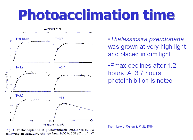
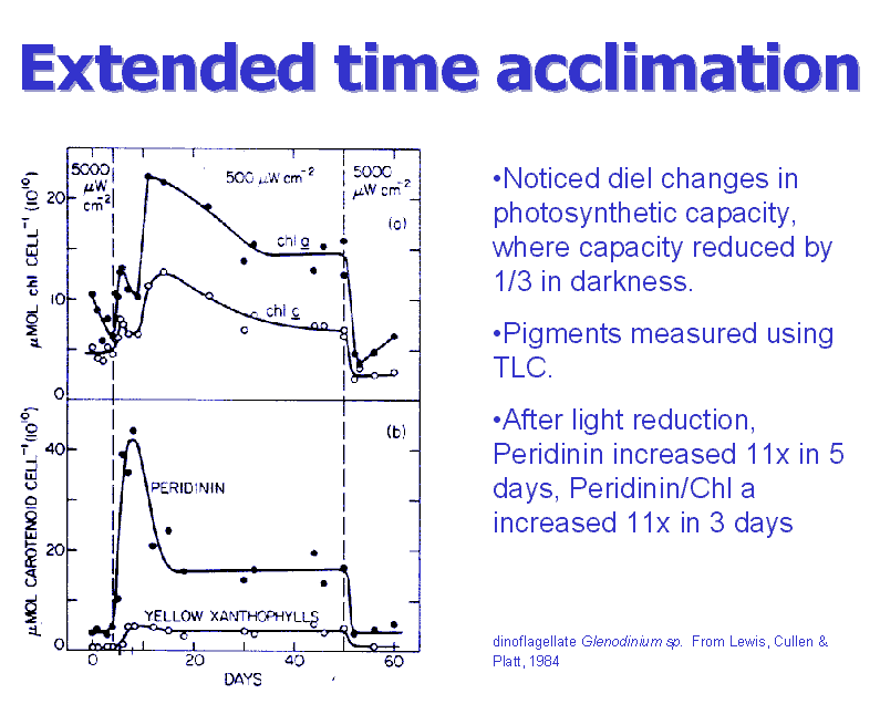
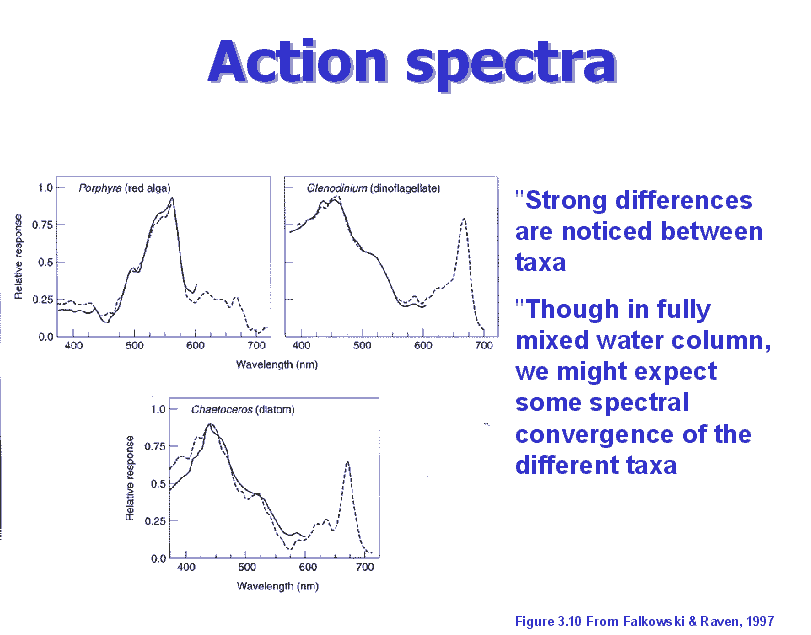
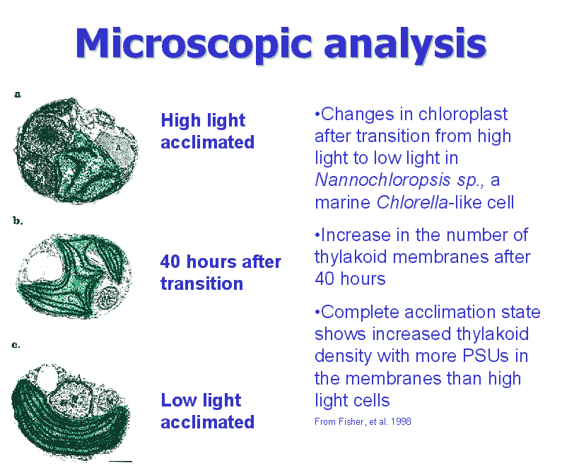
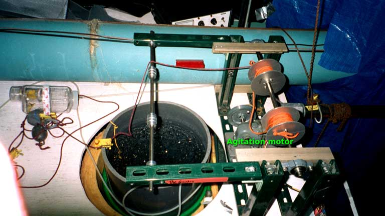
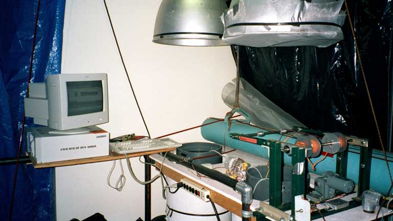
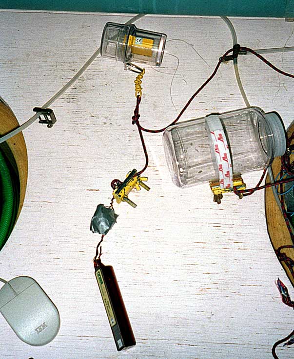
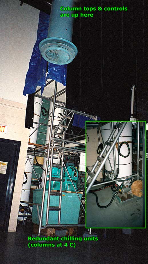
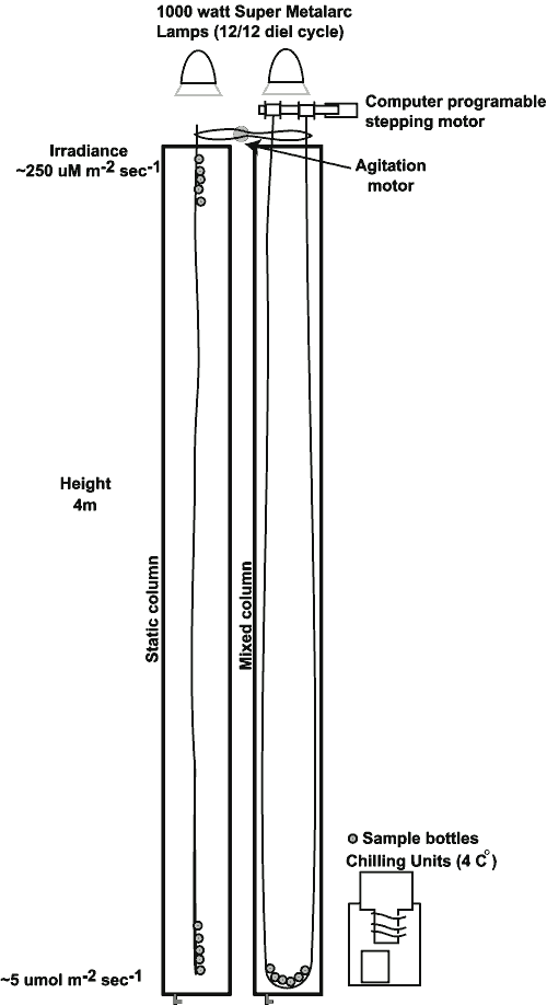
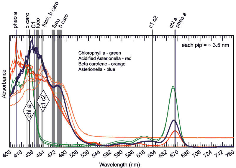
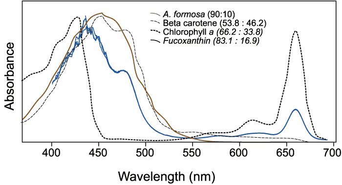